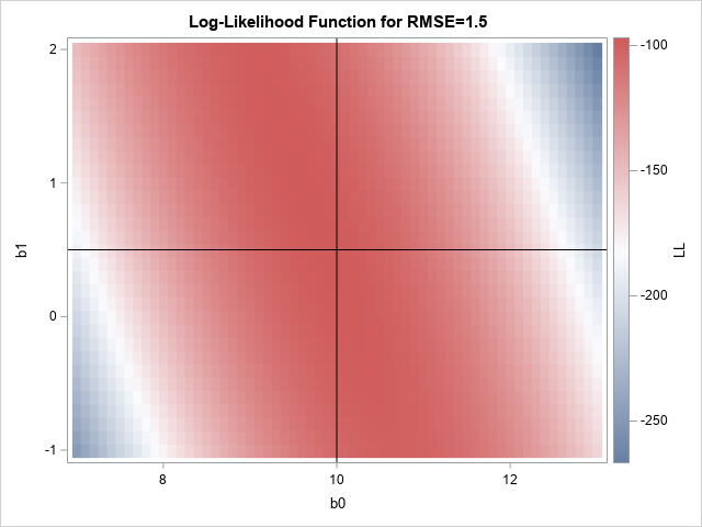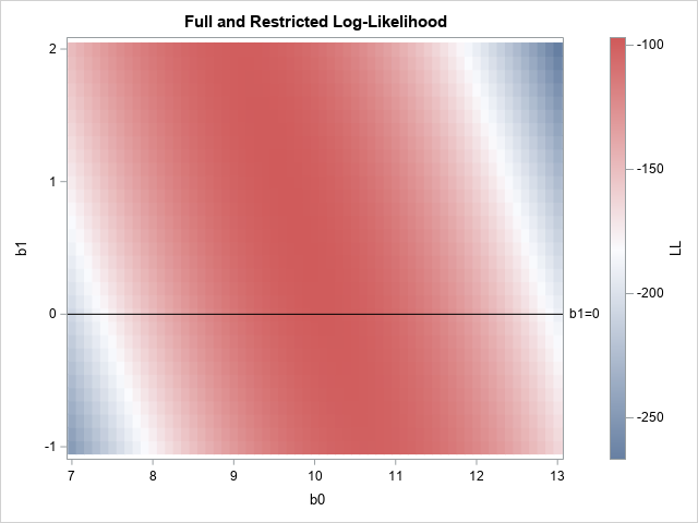
A recent article describes how to estimate coefficients in a simple linear regression model by using maximum likelihood estimation (MLE). One of the nice properties of an MLE formulation is that you can compare a large model with a nested submodel in a natural way. For example, if you can
Tag: linear regression
A statistical analyst used the GENMOD procedure in SAS to fit a linear regression model. He noticed that the table of parameter estimates has an extra row (labeled "Scale") that is not a regression coefficient. The "scale parameter" is not part of the parameter estimates table produced by PROC REG
A previous article discusses standardized coefficients in linear regression models and shows how to compute standardized regression coefficients in SAS by using the STB option on the MODEL statement in PROC REG. It also discusses how to interpret a standardized regression coefficient. Recently, a SAS user wanted to know how
For a linear regression model, a useful but underutilized diagnostic tool is the partial regression leverage plot. Also called the partial regression plot, this plot visualizes the parameter estimates table for the regression. For each effect in the model, you can visualize the following statistics: The estimate for each regression
An early method for robust regression was iteratively reweighted least-squares regression (Huber, 1964). This is an iterative procedure in which each observation is assigned a weight. Initially, all weights are 1. The method fits a least-squares model to the weighted data and uses the size of the residuals to determine
If you are thinking that nobody in their right mind would implement a Calculator API Service with a machine learning model, then yes, you’re probably right. But considering curiosity is in my DNA, it sometimes works this way and machine learning is fun. I have challenged myself to do it,
SAS' Udo Sglavo interviews colleague Jan Chvosta, director of Scientific Computing at SAS, on regression analysis and how it works.
One of the benefits of using the SWEEP operator is that it enables you to "sweep in" columns (add effects to a model) in any order. This article shows that if you use the SWEEP operator, you can compute a SSCP matrix and use it repeatedly to estimate any linear
In a previous article, I discussed various ways to solve a least-square linear regression model. I discussed the SWEEP operator (used by many SAS regression routines), the LU-based methods (SOLVE and INV in SAS/IML), and the QR decomposition (CALL QR in SAS/IML). Each method computes the estimates for the regression
In computational statistics, there are often several ways to solve the same problem. For example, there are many ways to solve for the least-squares solution of a linear regression model. A SAS programmer recently mentioned that some open-source software uses the QR algorithm to solve least-squares regression problems and asked
A previous article discusses how to interpret regression diagnostic plots that are produced by SAS regression procedures such as PROC REG. In that article, two of the plots indicate influential observations and outliers. Intuitively, an observation is influential if its presence changes the parameter estimates for the regression by "more
When you fit a regression model, it is useful to check diagnostic plots to assess the quality of the fit. SAS, like most statistical software, makes it easy to generate regression diagnostics plots. Most SAS regression procedures support the PLOTS= option, which you can use to generate a panel of
I've previously written about how to generate all pairwise interactions for a regression model in SAS. For a model that contains continuous effects, the easiest way is to use the EFFECT statement in PROC GLMSELECT to generate second-degree "polynomial effects." However, a SAS programmer was running a simulation study and
I previously showed how to create a decile calibration plot for a logistic regression model in SAS. A decile calibration plot (or "decile plot," for short) is used in some fields to visualize agreement between the data and a regression model. It can be used to diagnose an incorrectly specified
A previous article discusses the confidence band for the mean predicted value in a regression model. The article shows a "graded confidence band plot," which I saw in Claus O. Wilke's online book, Fundamentals of Data Visualization (Section 16.3). It communicates uncertainty in the predictions. A graded band plot is
You've probably seen many graphs that are similar to the one at the right. This plot shows a regression line overlaid on a scatter plot of some data. Given a value for the independent variable (x), the regression line gives the best prediction for the mean of the response variable
A previous article discussed how to solve regression problems in which the parameters are constrained to be a specified constant (such as B1 = 1) or are restricted to obey a linear equation such as B4 = –2*B2. In SAS, you can use the RESTRICT statement in PROC REG to
A data analyst recently asked a question about restricted least square regression in SAS. Recall that a restricted regression puts linear constraints on the coefficients in the model. Examples include forcing a coefficient to be 1 or forcing two coefficients to equal each other. Each of these problems can be
A previous article shows how to interpret the collinearity diagnostics that are produced by PROC REG in SAS. The process involves scanning down numbers in a table in order to find extreme values. This can be a tedious and error-prone process. Friendly and Kwan (2009) compare this task to a
A SAS programmer wanted to create a graph that illustrates how Deming regression differs from ordinary least squares regression. The main idea is shown in the panel of graphs below. The first graph shows the geometry of least squares regression when we regress Y onto X. ("Regress Y onto X"
In a previous article, I showed how to perform collinearity diagnostics in SAS by using the COLLIN option in the MODEL statement in PROC REG. For models that contain an intercept term, I noted that there has been considerable debate about whether the data vectors should be mean-centered prior to
I was recently asked about how to interpret the output from the COLLIN (or COLLINOINT) option on the MODEL statement in PROC REG in SAS. The example in the documentation for PROC REG is correct but is somewhat terse regarding how to use the output to diagnose collinearity and how
When fitting a least squares regression model to data, it is often useful to create diagnostic plots of the residuals versus the explanatory variables. If the model fits the data well, the plots of the residuals should not display any patterns. Systematic patterns can indicate that you need to include
A previous article describes the DFBETAS statistics for detecting influential observations, where "influential" means that if you delete the observation and refit the model, the estimates for the regression coefficients change substantially. Of course, there are other statistics that you could use to measure influence. Two popular ones are the
My article about deletion diagnostics investigated how influential an observation is to a least squares regression model. In other words, if you delete the i_th observation and refit the model, what happens to the statistics for the model? SAS regression procedures provide many tables and graphs that enable you to
For linear regression models, there is a class of statistics that I call deletion diagnostics or leave-one-out statistics. These observation-wise statistics address the question, "If I delete the i_th observation and refit the model, what happens to the statistics for the model?" For example: The PRESS statistic is similar to
Modern statistical software provides many options for computing robust statistics. For example, SAS can compute robust univariate statistics by using PROC UNIVARIATE, robust linear regression by using PROC ROBUSTREG, and robust multivariate statistics such as robust principal component analysis. Much of the research on robust regression was conducted in the
Have you ever run a regression model in SAS but later realize that you forgot to specify an important option or run some statistical test? Or maybe you intended to generate a graph that visualizes the model, but you forgot? Years ago, your only option was to modify your program
Deming regression (also called errors-in-variables regression) is a total regression method that fits a regression line when the measurements of both the explanatory variable (X) and the response variable (Y) are assumed to be subject to normally distributed errors. Recall that in ordinary least squares regression, the explanatory variable (X)
I remember the first time I used PROC GLM in SAS to include a classification effect in a regression model. I thought I had done something wrong because the parameter estimates table was followed by a scary-looking note: Note: The X'X matrix has been found to be singular, and a