A recent article describes how to estimate coefficients in a simple linear regression model by using maximum likelihood estimation (MLE). One of the nice properties of an MLE formulation is that you can compare a large model with a nested submodel in a natural way. For example, if you can fit the regression model y = β0 + β1 x + ε by optimizing the log-likelihood function, then you can fit the submodel y = β0 + ε simply by restricting the optimization to the parameter subspace where β1=0. Here ε ~ N(0, σ) is a vector of independent random normal errors whose magnitude is determined by the scale parameter σ > 0.

The restriction of the log-likelihood function to a lower dimensional subspace has a nice geometric interpretation. It is also the basis for the likelihood ratio (LR) test, which enables you to compare two related models and decide whether adding more parameters are results in a better model.

This article uses SAS to illustrate two methods to compute the likelihood ratio test for nested linear regression models. The first method calls the GENMOD procedure twice and uses a DATA step to compute the LR test. The second method computes the LR test from "first principles" by using a SAS IML program.

Nested OLS models

Before we discuss submodels in an MLE context, let's briefly review submodels for ordinary least squares (OLS) regression. A previous article discusses the geometry and formulation of a restricted regression model by using the RESTRICT statement in PROC REG. Both the RESTRICT statement and the TEST statement in PROC REG enable you to compare a model that has many parameters with a submodel that has one or more restrictions on the parameters.

In PROC REG, you can use the TEST statement to test a null hypothesis that the submodel (often called a reduced model) is just as valid as the full model. PROC REG runs an F test to potentially reject the null hypothesis. I don't want to discuss the details of linear models, but essentially the test statistic is a ratio. The numerator is the difference between the sums-of-squares of the reduced model and the denominator is the sum-of-squares for the full model. There are also some scaling factors; for details see the Penn State "STAT 501" lecture notes.

Nested MLE models

The formula for the log-likelihood function of the simple regression model is discussed in a previous article. If you define $r_i = y_ i-x_i \beta$, then the log-likelihood function is
$\mathit{ll}(\beta, \sigma; y, x) = -\frac{1}{2} \left[ n \log( \sigma^2 ) + n \log (2 \pi ) + \sum_i \frac{r^2}{\sigma^2 } \right]$
For the simple linear regression model, the parameters are (β0, β1, σ).

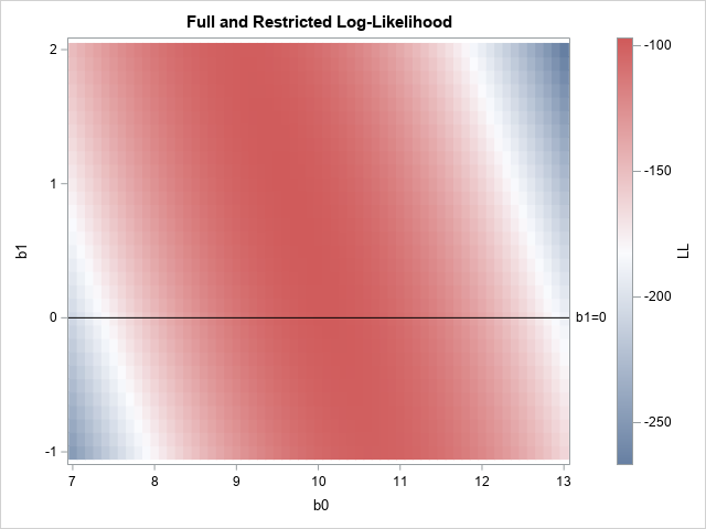
When you use MLE to fit nested models, you can use geometry to visualize the restricted (or reduced) log-likelihood function. For example, the graph to the right shows a heat map for the full log-likelihood function for a data set (N=50) that is simulated from the model with (β0, β1, σ)=(10, 0.5, 1.5). The colors correspond to the height of the function for each pair of estimates (b0, b1) when the scale parameter (σ) has the value σ = 1.5.

The linear subspace where b1=0 is shown as a black horizontal line. If you slice the graph of the log-likelihood function along the line, you obtain the reduced log-likelihood function as a cross-section of the full function, as shown below:

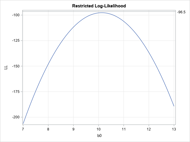
In the full model (the heat map), the largest value of the function (for σ=1.5) is -97.11 at (b0, b1) = (9.7, 0.8). If you restrict b1 to the line where b1=0, then the restricted log-likelihood (LL) function has a smaller maximum value. For the restricted LL function, the maximum value is -97.66 at (b0, b1) = (10.1, 0).

The likelihood ratio test

In the previous section, the log-likelihood values for the full and reduced models are similar. Consequently, you might wonder whether there is any significant advantage to using the full model (three free parameters) over the reduced model (two free parameters because b1=0).

In PROC REG, you can use the TEST statement to test the null hypothesis that β1=0. If the test rejects the null hypothesis, then the full model is significantly better. If the test fails to reject, then you might as well use the simpler reduced model to describe the data.

In the MLE framework, you can use the likelihood ratio test to compare a complex (full) model to any nested submodel. You must compute two quantities:

• Compute LL_F, the maximum value of the full log-likelihood function. This is sometimes called the unrestricted maximum likelihood value.
• Compute LL_R, the maximum value of the restricted log-likelihood function. This is sometimes called the restricted maximum likelihood value.

The likelihood ratio test uses the statistic
    LR = 2(LL_F – LL_R)
If you assume that the MLE estimates are asymptotically normal (and a few other assumptions, as explained in the StatLect notes about the likelihood ratio test), then the test statistic follows a chi-squared distribution with r degrees of freedom, where r is the difference between the number of free parameters in the full and reduced models. (Note: I like to I use the test statistic 2*abs(LL_F – LL_R), which doesn't require keeping track of which value is for the full model and which is for the reduced model.) In the simple regression example, there are three free parameters in the full model and two free parameters in the reduced model, so r=1, and you should compare the test statistic to a critical value for the chi-squared distribution with 1 degree of freedom.

The next sections show two ways to carry out the likelihood ratio (LR) test in SAS. The first method runs PROC GENMOD two times and uses the DATA step to compute the likelihood ratio test, as described in this SAS Note about the likelihood ratio test. The second method is is a "manual" computation in SAS IML that shows exactly how the LR test works.

Notice that the LR test uses the difference of two log-likelihood values. The likelihood ratio test gets its name because the difference between two log-likelihoods is equal to the logarithm of the ratio of the likelihoods.

The likelihood ratio test by using PROC GENMOD

Let's analyze a full and reduced model for the simulated data (called Sim) from the previous article about MLE for linear regression models.

The following SAS program calls PROC GENMOD twice, first for the full model and then again for the reduced (nested) submodel. For both calls, the ModelFit table is written to a data set. The ModelFit table contains the log-likelihood (LL) value at the parameter estimates in the 6th row, and also contains the error degrees of freedom for the full and reduced models. You can then use a DATA step to read the LL values and to form the test statistic 2*abs(LL_F – LL_R). You can then compare the test statistic with the critical value of the chi-squared distribution with the appropriate degrees of freedom. Since the test will provide a one-sided p-value, you can use the SDF function instead of computing (1 – CDF) to obtain the right-tail probability.

/* Call PROC GENMOD twice and use DATA step to compute LR test.
   See https://support.sas.com/kb/24/474.html */
proc genmod data=Sim plots=none;
   Full: model y = x;
   ods select ModelFit;
   ods output ModelFit=LLFull;
run;
proc genmod data=Sim plots=none;
   Reduced: model y = ;
   ods select ModelFit;
   ods output ModelFit=LLRed;
run;
 
/* "Full Log Likelihood" is the 6th row in the data set */
data LRTest;
retain DF;
keep DF LLFull LLRed LRTest pValue;
merge LLFull(rename=(DF=DFFull Value=LLFull))
      LLRed (rename=(DF=DFRed  Value=LLRed));
if _N_ = 1 then
   DF = DFRed - DFFull;
if _N_ = 6 then do;
   LRTest = 2*abs(LLFull - LLRed);     /* test statistic */
   pValue = sdf("ChiSq", LRTest, DF);  /* p-value Pr(X > LRTest) where X~ChiSq(DF) */
   output;
end;
label LLFull='LL Full' LLRed='LL Red' LRTest='LR Test' pValue = 'Pr > ChiSq';
run;
 
proc print data=LRTest noobs label;
run;

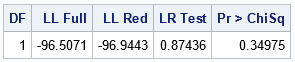
The likelihood-ratio test statistic is 0.87436. In the chi-squared distribution with 1 degree of freedom, the probability is about 0.35 that a random variate is to the right of this value. Because this probability is greater than 0.05, you should not reject the null hypothesis that the reduced model (β1=0) explains the data better than the full model. Therefore, use the reduced model for these data.

The Appendix shows the same computation performed "manually" in SAS IML by optimizing the log-likelihood function for the full and reduced models. The Appendix shows that you get the same values for the LR test.

Summary

This article shows how to use SAS to perform a likelihood ratio test for nested linear regression models. The example in the body of the article calls the GENMOD procedure twice and uses a DATA step to compute the LR test. The Appendix shows a second method, which is to compute the LR test from "first principles" by using a SAS IML program to optimize the full and reduced likelihood functions.

Although the example in this article is a linear regression model, the general idea applies to other nested models. For a description of the general case, see the StatLect lecture notes.

Appendix: The likelihood ratio test from first principles

You can use PROC IML in SAS to compute the LR test from "first principles" by using a SAS IML program to optimize the full and reduced likelihood functions. The example uses the same simulated data (called Sim) as the rest of the article. The data are defined in the previous article about MLE for linear regression models.

The first step is to find the parameter values that maximize the log-likelihood (LL) function for the full model and to evaluate the LL function at the optimal value. This was done in the previous article, but it is repeated below:

proc iml;
/* the data are defined in 
   https://blogs.sas.com/content/iml/2024/03/20/mle-linear-regression.html
*/
use Sim;
   read all var {"x" "y"};
close;
X = j(nrow(x),1,1) || x;    * design matrix;
 
/* the three-parameter model (beta0, beta1, sigma) */
start LogLikRegFull(parm) global(X, y);
   pi = constant('pi');
   b = parm[1:2];
   sigma = parm[3];
   sigma2 = sigma##2;
   r = y - X*b;
   LL = sum( logpdf("normal", r, 0, sigma) );    
   return LL;
finish;
 
/* max of LogLikRegFull, starting from param0 */
start MaxLLFull(param0)  global(X, y);
   /*     b0 b1 sigma constraint matrix */
   con = { .   . 1E-6,    /* lower bounds: none  for beta[i]; 0 < sigma */
           .   . .};      /* upper bounds: none */
   opt = {1,              /* find maximum of function   */
          0};             /* do not print durin optimization */
   call nlpnra(rc, z, "LogLikRegFull", param0, opt, con);
   return z;
finish;
 
param0 = {11 1 1.2};     /* initial guess for full model */
MLFull = MaxLLFull( param0 );
LLF = LogLikRegFull(MLFull);  /* LL at the optimal parameter */
print LLF[F=8.4], MLFull[c={'b0' 'b1' 'RMSE'} F=7.5];

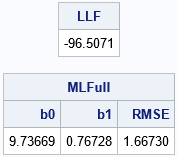
The maximum LL value for the full model is LL_F = -96.507. We know that restricting the domain of the LL function will result in a smaller optimal value, but we have previously seen the graph of the restricted LL function, and we know that the maximum value of the restricted LL function is only slightly smaller. The following SAS IML statements find the optimal parameter values for the reduced model and evaluate the restricted LL function:

/* the two-parameter model (beta0, 0, sigma) */
start LogLikRegRed(parm) global(X, y);
   p = parm[1] || 0 || parm[2];
   return( LogLikRegFull( p ) );
finish;
/* max of LogLikRegReded, starting from param0 */
start MaxLLRed(param0)  global(X, y);
   /*     b0 sigma constraint matrix */
   con = { .  1E-6,       /* lower bounds: none  for beta[i]; 0 < sigma */
           .  .};         /* upper bounds: none */
   opt = {1,              /* find maximum of function   */
          0};             /* do not print durin optimization */
   call nlpnra(rc, z, "LogLikRegRed", param0, opt, con);
   return z;
finish;
 
param0 = {11 1.2};   /* initial guess */
MLRed = MaxLLRed( param0 );
/* what is the LL at the optimal parameter? */
LLR = LogLikRegRed(MLRed);
print LLR[F=8.4], MLRed[c={'b0' 'b1' 'RMSE'} F=7.5];

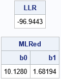
The maximum LL for the reduced model is LL_R = -96.944. From these two values, you can construct the test statistic for the likelihood ratio test. You can then compare the test statistic with the critical value of the chi-squared distribution with 1 degree of freedom. Since the test will provide a one-sided p-value, you can use the SDF function instead of computing (1 – CDF) to obtain the right-tail probability:

/* LL ratio test for null hypothesis of restricted model  */
LLRatio = 2*abs(LLF - LLR);         /* test statistic */
DF = 1;
pValue = sdf('ChiSq', LLRatio, DF); /* Pr(z > LLRatio) if z ~ ChiSq with DF=1 */
print DF LLF LLR LLRatio[F=7.5] pValue[F=PVALUE6.4];

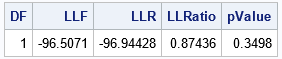
The manual implementation of the likelihood-ratio test is the same as provided by running PROC GENMOD twice. The test statistic of 0.87436 has a p-value about 0.35. Again, the test suggests that you reject the null hypothesis. The reduced regression model that has β1=0 is sufficient to explain the data.