Tips for computing right-tail probabilities and quantiles

A colleague was struggling to compute a right-tail probability for a distribution. Recall that the cumulative distribution function (CDF) is defined as a left-tail probability. For a continuous random variable, X, with density function f, the CDF at the value x is
F(x) = Pr(X ≤ x) = ∫ f(t) dt
where the integral is evaluated on the interval (-∞, x). That is, it is the area under the density function "to the left" of x. In contrast, the right-tail probability is the complement of this quantity. The right-tail probability is defined by
S(x) = Pr(X ≥ x) = 1 – F(x)
It is the area under the density function "to the right" of x.

The right-tail probability is also called the right-side or upper-tail probability. The function, S, that gives the right-tail probability is called the survival distribution function (SDF). Similarly, a quantile that is associated with a probability that is close to 0 or 1 might be called an extreme quantile. This article discusses why a naive computation of an extreme quantile can be inaccurate. It shows how to compute extreme probabilities and extreme quantiles by using special functions in SAS:

The SDF function computes a right-tail probability.
the SQUANTILE function computes an extreme quantile for p ≈ 1.

Accurate computations of extreme probabilities

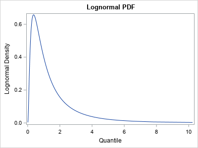
My colleague contacted me to discuss some issues related to computing an extreme quantile for p ≈ 1. To demonstrate, I will use the standard lognormal distribution, whose PDF is shown to the right. (However, this discussion applies equally well to other distributions.) When p is small, the lognormal quantile is close to 0. When p is close to 1, the lognormal quantile is arbitrarily large because the lognormal distribution is unbounded.

The following SAS DATA step uses the QUANTILE function to compute extreme quantiles in the left and right tails of the lognormal distribution. The quantiles are associated with the probabilities p=1E-k and p=1 – 1E-k for k=8, 9, 10, ..., 15.

%let Distrib = Lognormal;
data Have;
do pow = -8 to -15 by -1;
   p = 10**pow;                   
   Lx = quantile("&Distrib", p);   /* left-tail quantile: find x such that CDF(x) = p */
   Rp = 1 - p;                     /* numerically, 1-p = 1 for p < MACEPS */
   Rx = quantile("&Distrib", Rp);  /* right-tail quantile: find x such that CDF(x) = 1-p */
   output;
end;
format Rp 18.15;
run;
 
proc print noobs; run;

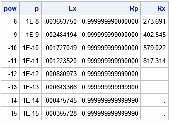
The second column shows the probability, p, and the Lx column shows the corresponding left-tail quantile. For example, the first row shows that 1E-8 is the probability that a standard lognormal random variate has a value less than 0.00365. The Rp column shows the probability 1 – p. The Rx column shows the corresponding quantile. For example, the first row shows that 1 – 1E-8 is the probability that a standard lognormal random variate has a value greater than 273.691.

From experimentation, it appears that the QUANTILE function returns a missing value when the probability argument is greater than or equal to 1 – 1E-12. The SAS log displays a note that states
NOTE: Argument 2 to function QUANTILE('Normal',1) at line 5747 column 9 is invalid.
This means that the function will not compute extreme-right quantiles. Why? Well, I can think of two reasons:

When p is very small, the quantity 1 – p does not have full precision. (This is called the "loss-of-precision problem" in numerical analysis.) In fact, if p is less than machine epsilon, the expression 1 – p EXACTLY EQUALS 1 in floating-point computations! Thus, we need a better way to specify probabilities that are close to 1.
For unbounded distributions, the CDF function for an unbounded distribution is extremely flat for values in the right tail. Because the pth quantile is obtained by solving for the root of the function CDF(x) - p = 0, the computation to find an accurate extreme-right quantile is numerically imprecise for unbounded distributions.

Compute extreme quantiles in SAS

The previous paragraph does not mean that you can't compute extreme-right quantiles. It means that you should use a function that is specifically designed to handle probabilities that are close to 1. The special function is the SQUANTILE function, which uses asymptotic expansions and other tricks to ensure that extreme-right quantiles are computed accurately. If x is the value returned by the SQUANTILE function, then 1 – CDF(x) = p. You can, of course, rewrite this expression to see that x satisfies the equation CDF(x) = 1 – p.

The syntax for the SQUANTILE function is almost the same as for the QUANTILE function. For any distribution, QUANTILE("Distrib", 1-p) = SQUANTILE("Distrib", p). That is, you add an 'S' to the function name and replace 1 – p with p. Notice that by specifying p instead of 1 – p, the right-tail probability can be specified more accurately.

The following SAS DATA step is a modification of the previous DATA step. It uses the SQUANTILE function to compute the extreme-right quantiles:

data Want;
do pow = -8 to -15 by -1;
   p = 10**pow;
   Lx = quantile("&Distrib", p);   /* find x such that CDF(x) = p */
   Rp = 1 - p;
   Rx = squantile("&Distrib", p);  /* find x such that 1-CDF(x)=p */
   output;
end;
format Rp 18.15;
drop pow;
run;
 
proc print noobs; run;

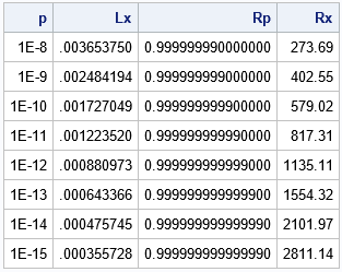
The table shows that the SQUANTILE function can compute quantiles that are far in the right tail. The first row of the table shows that the probability is 1E-8 that a lognormal random variate exceeds 273.69. (Equivalently, 1 – 1E-8 is the probability that the variate is less than 273.69.) The last row of the table shows that 1E-15 is the probability that a lognormal random variate exceeds 2811.14.

Compute extreme probabilities in SAS

When p is small, the "loss-of-precision problem" (representing 1 – p in finite precision) also affects the computation of the cumulative probability (CDF) of a distribution. That is, the expression CDF("Distrib", 1-p) might not be very accurate because 1 – p loses precision when p is small. To counter that problem, SAS provides the SDF function, which computes the survival distribution function (SDF). The SDF returns the right-tail quantile x for which 1 – CDF(x) = p. This is equivalent to finding the left-tail quantile that satisfies CDF(x) = 1 – p.

The following DATA step computes several one-sided probabilities. For each value of x, the program computes the probability that a random lognormal variate is greater than x:

%let Distrib = lognormal;
data SDF;
do x = 500 to 2500 by 500;              /* extreme quantiles  */
   Rp       = 1 - cdf("&Distrib", x);   /* right-tail probability */
   RpBetter = sdf("&Distrib", x);       /* better computation of right-tail probability */
   output;
end;
run;
 
proc print noobs; run;

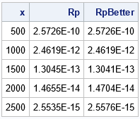
The difference between the probabilities in the Rp and RpBetter columns are not as dramatic as for the quantiles in the previous section. That is because the quantity 1 – CDF(x) does not lose precision when x is large because CDF(x) ≈ 1. Nevertheless, you can see small differences between the columns, and the RpBetter column will tend to be more accurate when x is large.

Summary

This article shows two tips for working with extreme quantiles and extreme probabilities. When the probability is close to 1, consider using the SQUANTILE function to compute quantiles. When the quantile is large, consider using the SDF function to compute probabilities.

Blogs