In practice, there is no need to remember textbook formulas for the ANOVA test because all modern statistical software will perform the test for you. In SAS, the ANOVA procedure is designed to handle balanced designs (the same number of observations in each group) whereas the GLM procedure can handle unbalanced designs. Each procedure has a simple syntax which enables you to quickly produce an ANOVA table and test hypotheses such as whether the group means are equal.

However, every elementary textbook presents formulas for the cells in a one-way ANOVA table because there is value in understanding what each cell represents. For the statistics student, the formulas introduce important concepts in linear models, such as the sum of squares, mean squares, and the F statistic as a ratio of sums of squares. In addition, implementing a "manual" computation has value when teaching statistical programming. If a new programmer implements a familiar statistical test in a new language, she can easily compare her answers to the answers produced by standard ANOVA routines.

Recently, I taught a short course on the SAS IML language, which caused me to think about how to implement the ANOVA formulas in the SAS IML language. This article shares the computations and discusses techniques that are useful for the programming exercise.

To make the computations accessible to the largest number of students, I decided NOT to use the matrix formulation of ANOVA. Recall that the ANOVA test can be viewed as a linear regression model and solved by using least-squares matrix computations. This is a cool fact, but not everyone who takes a programming course is comfortable with matrix representations and linear algebra. Consequently, I choose to program the ANOVA by using a traditional sums-of-squares approach. For a matrix formulation, see Chapter 4 of the Penn State online textbook Analysis of Variance and Design of Experiments, which includes SAS IML programs for ANOVA computations.

Sample data for an ANOVA

The following DATA step and call to PROC ANOVA are taken from the "Getting Started" example in SAS documentation for the ANOVA procedure. The response variable is the nitrogen content (in mg) for six treatment groups of red clover plants. Each treatment group contains five plants that were inoculated with a particular strain of bacteria. The research question is to infer whether the group means are equal across all treatment groups.

title1 'Nitrogen Content of Red Clover Plants';
data Clover;
   input Strain $ Nitrogen @@;
   datalines;
3DOK1  19.4 3DOK1  32.6 3DOK1  27.0 3DOK1  32.1 3DOK1  33.0
3DOK5  17.7 3DOK5  24.8 3DOK5  27.9 3DOK5  25.2 3DOK5  24.3
3DOK4  17.0 3DOK4  19.4 3DOK4   9.1 3DOK4  11.9 3DOK4  15.8
3DOK7  20.7 3DOK7  21.0 3DOK7  20.5 3DOK7  18.8 3DOK7  18.6
3DOK13 14.3 3DOK13 14.4 3DOK13 11.8 3DOK13 11.6 3DOK13 14.2
COMPOS 17.3 COMPOS 19.4 COMPOS 19.1 COMPOS 16.9 COMPOS 20.8
;
/* sort groups so that we can use the UNIQUE function in IML later */
proc sort data=Clover;
   by Strain;
run;
 
proc means data=Clover Mean StdDev printalltypes;
   class Strain;
   var Nitrogen;
run;
proc anova data=Clover plots=BoxPlot;
   class Strain;
   model Nitrogen = Strain;
   ods select OverallANOVA BoxPlot;
run;

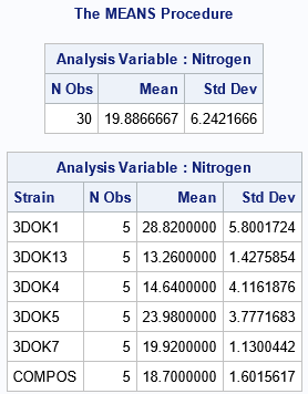
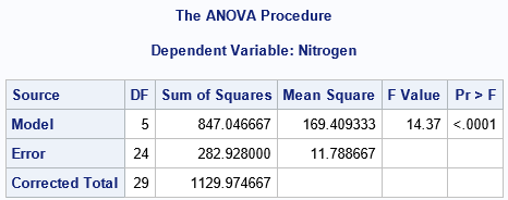
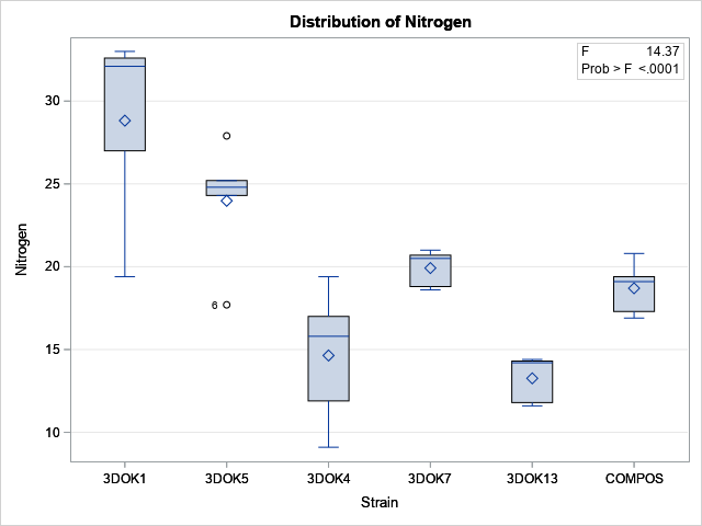
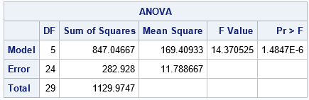
From the box plot, we suspect that the group means are NOT the same for the six groups. The output from PROC MEANS also suggests that the means of the groups are not similar, given the variation in the data within groups. The ANOVA test is for the null hypothesis that μ₁ = μ₂ = ... = μ₆, versus the alternative hypothesis that not all the means are equal. The F test in the ANOVA table has a p-value that is tiny, which indicates that we can reject the null hypothesis at the 0.05 significance level.

The sums of squares formulas for ANOVA

Recall that the ANOVA model assumes that the response variable (Y) in the i_th group can be modeled by using deviations from an overall mean:
Y_ij = μ + τ_i + ε_ij
where μ is the overall mean response (also called the "grand mean"), τ_i are the deviations of the group means from the overall mean (so Σ_i τ_i = 1), and the ε_ij is the error (or residual) of the j_th observation in the i_th group.

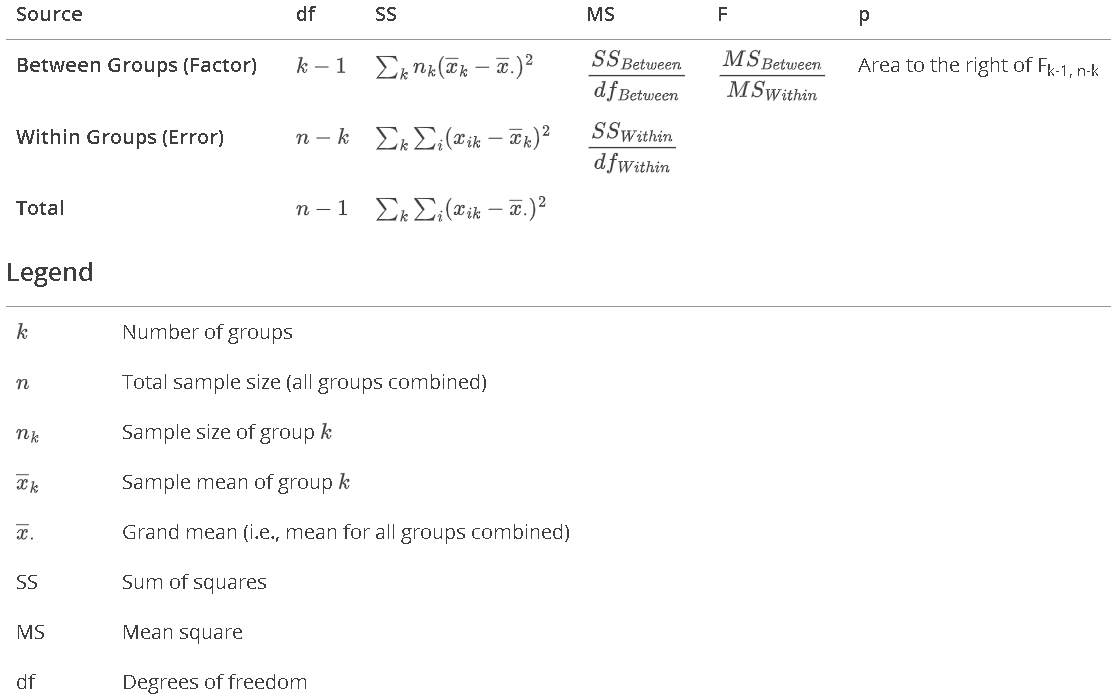
The SAS output uses "Model", "Error", and "Corrected Total" as the labels for the rows of the ANOVA output. Another common choice is "Between Groups", "Within Groups" and "Total", respectively. For medical trials, you might see "Treatment", "Error", and "Total". Whatever labels you use for the "Source" column, the first row represents the variation that is explained by the regression model that predicts the response variable from the group. The second row is the sum of squares of the residuals. The third row is the sum of the first two rows.

The web page for "One-Way ANOVA" in Penn State's "Stat 200: Elementary Statistics" course describes the sum-of-squares formulas that are used to create the ANOVA table. Notice that Penn State uses the "Between Groups" versus "Within Groups" notation.

Group processing in PROC IML

Before we can fill out the cells of the ANOVA table, we need to calculate four statistics: the total number of observations, the number in each subgroup, the overall mean, and the mean of each group. You can use either the UNIQUE-LOC trick or the UNIQUEBY technique to perform BY-group processing in the IML language. The UNIQUE-LOC trick is easier to understand, so let's use that method. The following call to PROC IML reads the data and computes the four preliminary statistics:

proc iml;
use Clover;
   read all var {'Strain'} into G;   /* group IDs */
   read all var {'Nitrogen'} into Y; /* response variable */
close;
 
nTotal = nrow(Y);      /* assume no missing values */
grandMean = mean(Y);
/* use UNIQUE-LOC technique to find group sizes and means */
u = unique(G);         /* levels of the CLASS variable */
k = ncol(u);           /* number of groups */
n = j(k, 1);           /* n[i] = size of each group */
mean = j(k, 1);        /* mean[i] = mean of each group */
do i = 1 to k;
   idx = loc(G=u[i]);  /* find obs in group */
   n[i] = ncol(idx);
   mean[i] = mean(Y[idx]);
end;
print nTotal grandMean, (n||mean)[r=u c={'n' 'mean'}];
QUIT;

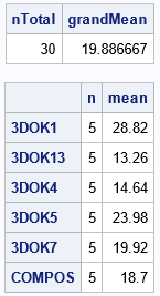
The output agrees with the output from PROC MEANS. Notice that the loop is over the number of groups, which is usually small. Within each iteration, the program calculates the size and mean of each group. For these data, the group sizes are the same, but the program can handle groups of different sizes.

Sums-of-squares and a manual ANOVA calculation

You can define a SAS IML module that uses the previous calculations to compute the preliminary statistics, then uses sum-of-squares computations to compute the remaining columns of the ANOVA table. The F statistic is the ratio of the model sum-of-squares and the error sum-of-squares. The p-value is a right-tail probability, so you can use the SDF function in SAS to compute that quantity accurately.

proc iml;
/* "Manually" calculate and display a one-way ANOVA table.
   Return a 3 x 5 ANOVA table. You can print the table by using 
   the following row headers and column headers:
   colNames = {"DF" "Sum of Squares" "Mean Square" "F Value" "Pr > F"};
   rowNames = {"Model", "Error", "Total"};
*/
start OneWayAnova(Response, Group);
   idx = loc(Response^=.); 
   if ncol(idx) < 2 then STOP "Invalid data";
   Y = Response[idx];    /* exclude missing values */
   G = Group[idx];       /* assume at least k=2 groups */
 
   nTotal = nrow(Y);      
   grandMean = mean(Y);
   /* use UNIQUE-LOC technique to find group sizes and means */
   u = unique(G);         /* levels of the CLASS variable in alphabetical order */
   k = ncol(u);           /* number of groups */
   n = j(k, 1);           /* n[i] = size of each group */
   mean = j(k, 1);        /* mean[i] = mean of each group */
   do i = 1 to k;
      idx = loc(G=u[i]);  /* find obs in group */
      n[i] = ncol(idx);
      mean[i] = mean(Y[idx]);
   end;
   /* DF calculations */
   DF_Model = k-1; 
   DF_Error = nTotal - k;
   DF_Total = DF_Model + DF_Error; 
 
   /* sum-of-squares computations */
   SS_Model = sum( n # (mean - grandMean)##2 );
   longMean = colvec( repeat(mean, n) );  /* see 2nd syntax for REPEAT function */
   SS_Error = ssq( Y - longMean );
   SS_Total = SS_Model + SS_Error;
 
   /* define vectors */
   DF = DF_Model // DF_Error // DF_Total;
   SS = SS_Model // SS_Error // SS_Total;
 
   /* mean square, F statistic,  and p-value */
   MS = SS / DF;
   MS[3] = .;
   FValue = MS[1] / MS[2];                         /* F statistic */
   ProbF  = sdf( "F", FValue, DF_Model, DF_Error); /* right-tail p value */
 
   /* put the results into a table */
   ANOVA = j(3,5, .);
   ANOVA[ ,1] = DF;
   ANOVA[ ,2] = SS;
   ANOVA[ ,3] = MS;
   ANOVA[1,4] = FValue;
   ANOVA[1,5] = ProbF;
   return ANOVA;
finish;
 
/* test on real data */
use Clover;
   read all var {'Strain'} into G;   /* group IDs */
   read all var {'Nitrogen'} into Y; /* response variable */
close;
ANOVA = OneWayAnova(Y, G);
/* If desired, display missing values as blanks. See
   https://blogs.sas.com/content/iml/2024/09/16/sas-display-missing-values.html */
stats = {"DF" "Sum of Squares" "Mean Square" "F Value" "Pr > F"};
source = {"Model", "Error", "Total"};
print ANOVA[c=stats r=source];

The output from the SAS IML function is equivalent to the OUTPUT from PROC ANOVA. The function can handle data for which the groups are different sizes, such as you might analyze by using PROC GLM. Notice a few tricks in the program:

• There are no loops other than one loop over groups.
• I used the SUM function to sum some quantities, but I used the SSQ function to compute the sum-of-squares for a vector of values.
• The REPEAT function has two important use cases. The function is usually used to replicate one or more values into a matrix. But the second syntax will "expand" a vector of values and frequencies into a long vector in which each value is replicated a specified number of times.
• I use the row labels "Model" and "Error", but you can substitute the terms "Between Groups" and "Within Groups," if you prefer.

Summary

SAS provides the ANOVA and GLM procedures to perform ANOVA tests. These procedures handle multi-way ANOVAs and support interaction effects. The SAS IML program in this article demonstrates how to use a matrix-vector programming like IML to duplicate the computations in a one-way ANOVA table. Professors might show this program to students in a statistics class. Instructors might use the program to demonstrate vectorized computations to programmers who are learning the SAS IML language. The program demonstrates a few programming techniques that are useful to know.