Maximum likelihood estimates for linear regression

A statistical analyst used the GENMOD procedure in SAS to fit a linear regression model. He noticed that the table of parameter estimates has an extra row (labeled "Scale") that is not a regression coefficient. The "scale parameter" is not part of the parameter estimates table produced by PROC REG or PROC GLM. In addition, PROC GENMOD displays a note that states,
Note: The scale parameter was estimated by maximum likelihood.
The analyst wanted to know how to interpret "the scale parameter" in the model.

This article reviews the MLE process for linear models and compares the output of PROC REG and PROC GENMOD. It shows how to use nonlinear optimization to optimize the log-likelihood function for the linear regression model, thus reproducing the GENMOD output.

Least square estimates versus maximum likelihood estimates

PROC GENMOD and PROC REG differ in the way that they estimate the coefficients of a linear regression model. PROC REG uses the method of ordinary least squares (OLS), which is a direct method. In contrast, PROC GENMOD uses maximum likelihood estimation (MLE), which is a general method that can apply to many regression models, not just linear models. As part of the MLE computation, the GENMOD procedure must estimate one parameter (the "scale parameter") that the OLS method does not estimate directly. Rather, OLS obtains the "scale parameter" as a consequence of the least squares process.

Both methods assume that the regression model has the matrix form Y = Xβ + ε, where ε is a vector of independent errors. Often, the errors are assumed to be normally distributed as N(0, σ).

The simplest linear regression model is for one continuous regressor: y = β0 + β1 x + ε. The following SAS DATA step simulates n=50 observations from this model for the parameter values (β0, β1, σ) = (10, 0.5, 1.5).

/* simple linear model 
   y ~ betas0 + beta1*x + eps for eps ~ N(0,sigma)
*/
data Sim;
call streaminit(4321);
array beta[0:1] (10, 0.5);     /* beta0=10; beta1 = 0.5 */
sigma = 1.5;                   /* scale for the distribution of errors */
N = 50;
do i = 1 to N;
   x = i / N;                  /* X is equally spaced in [0,1] */
   eta = beta[0] + beta[1]*x;  /* model */
   y =  eta + rand("Normal", 0, sigma);
   output;
end;
run;

The next sections analyze these simulated data twice: first by using OLS, then by using MLE.

PROC REG and least squares estimates

The OLS method estimates the regression coefficients by solving the normal equations (X'X)b = X`Y for b. The predicted values are X*b, and the residuals are r = Y - X*b. If you assume that the model is correctly specified and the error terms are normally distributed, you can estimate σ from the distribution of the residuals. PROC REG and other SAS procedures first estimate the sum of squared errors (SSE) as Σ r_i², then estimate σ as the root mean squared error (RMSE), which is sqrt(SSE/(n-p)), where n is the number of observations and p is the number of regression parameters. Thus, I often think of the OLS method as a two-step method: first, estimate the β coefficients, then use those values to estimate σ as the RMSE.

The following call to PROC REG produces OLS estimates for the simulated data.

proc reg data=Sim plots(only)=fit;
   model y = x;
run;

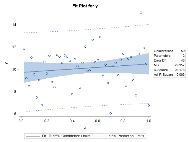
The call to PROC REG produces a fit plot that enables you to visualize the fit. The vertical distances from the markers to the regression line are the (absolute) residuals. The procedure outputs the parameter estimates and the RMSE statistic, which estimates σ:

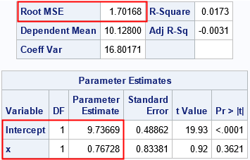
I have highlighted a few rows of output. Recall that the data are a random sample of size n=50 from a model whose parameters are (β0, β1, σ) = (10, 0.5, 1.5). The parameter estimates are (9.7, 0.77, 1.7), which are close to the parameter values. The next section uses PROC GENMOD to obtain the MLE estimates for the same parameters.

PROC GENMOD and maximum likelihood estimates

In contrast to the "two step" OLS method, the MLE method estimates σ and the β coefficients simultaneously. Look at the output from the following call to PROC GENMOD:

proc genmod data=Sim plots=none;
   model y = x;
run;

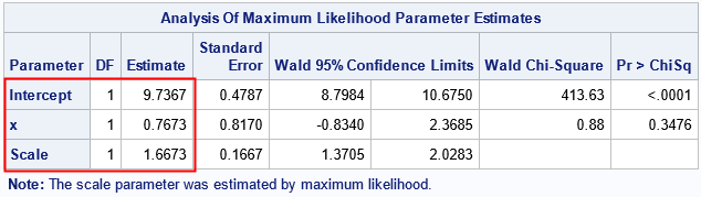
Notice that the output from PROC GENMOD includes the estimate for the scale of the error distribution as part of the parameter estimates table. The output also includes a NOTE that reminds you that the scale parameter was estimated as part of the solution. In this table, the estimates for the regression coefficients ("the betas") are the same as for PROC REG (to four decimals), but the estimate of the scale parameter is smaller. This will always be the case. Recall that the least square method estimates σ as sqrt(SSE/(n-p)), where n is the number of observations and p is the number of regression parameters. In contrast, the MLE method uses sqrt(SSE/(n), which is the "population" formula for the standard deviation of the residuals. (Recall that the population standard deviation has n in the denominator whereas the sample standard deviation uses n-1.) Thus, the MLE method uses a larger denominator, which makes the estimate smaller than the OLS estimate.

PROC GENMOD also outputs a table that shows some goodness-of-fit statistics:

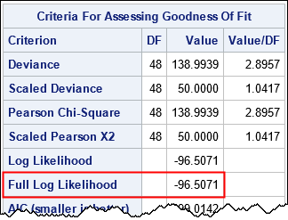
I've highlighted the value of the log-likelihood function evaluated at the parameter estimates. The next section shows how to construct the log-likelihood function for a linear regression model.

MLE for linear regression from first principles

You can find online descriptions of the maximum likelihood equations for linear regression. For the linear model, you can explicitly solve for the parameter values that maximize the log-likelihood function. The MLE estimates for the regression coefficients are the same as for the least squares method; the estimate for the scale parameter is always the (population) standard deviation of the residuals. Consequently, you can obtain the MLE estimates "directly" by using the least squares solution. However, for the sake of demonstrating how the MLE estimates are computed in PROC GENMOD, this section constructs the log-likelihood function for the linear regression model and finds performs nonlinear optimization to find the parameter values that maximize the log likelihood.

The log-likelihood function is a function of the coefficients, β, and of the unknown parameter, σ, which is the scale parameter for the "noise" or the magnitude of the error term. It requires the data value to evaluate the function. If you assume normally distributed errors, the MLE equations are (see the StatLect notes):
$\mathit{ll}(\beta, \sigma; y, x) = -\frac{1}{2} \sum_i \left[ \frac{(y_ i-x_i \beta)^2}{\sigma^2 } + \log( \sigma^2 ) + \log (2 \pi ) \right]$

If you define $r_i = y_ i-x_i \beta$ , then the equation becomes
$\mathit{ll}(\beta, \sigma; y, x) = -\frac{1}{2} \left[ n \log( \sigma^2 ) + n \log (2 \pi ) + \sum_i \frac{r^2}{\sigma^2 } \right]$
Because the scale parameter appears as σ², sometimes the variance is used as the scale parameter in the MLE equations. However, PROC GENMOD uses σ, and I will do the same.

It is instructive to "manually" maximize the likelihood function, given the data. You can type in the previous formula, but the simpler way is to sum the SAS-supplied LOGPDF function for the normal distribution, as discussed in a previous article.

proc iml;
use Sim;        /* read the data */
   read all var {"x" "y"};
close;
X = j(nrow(x),1,1) || x;    * design matrix;
 
start LogLikReg(parm) global(X, y);
   pi = constant('pi');
   b = parm[1:2];
   sigma = parm[3];
   sigma2 = sigma##2;
   r = y - X*b;
   /* you can use the explicit formula:
         n = nrow(X);
         LL = -1/2*(n*log(2*pi) + n*log(sigma2) + ssq(r)/sigma2);  
      but a simpler expression uses the sum of the log-PDF */
   LL = sum( logpdf("normal", r, 0, sigma) );                
   return LL;
finish;

If you draw a heat map of the log-likelihood function for σ=1.5, you get the following picture. From the heat map, you can guess that the log-likelihood function achieve a maximum somewhere close to the center of the graph. For reference, I have overlaid lines at the parameter values (β0, β1) = (10, 0.5).

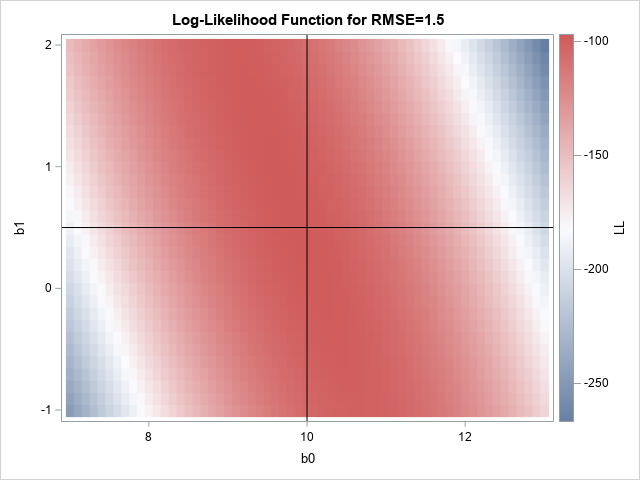
The graph suggests reasonable values for an initial guess for a nonlinear optimization. The following call to the NLPNRA subroutine in SAS IML performs the maximum likelihood optimization:

/* set constraint matrix, options, and initial guess for optimization */
/*     b0 b1 sigma constraint matrix */
con = { .   . 1E-6,    /* lower bounds: none  for beta[i]; 0 < sigma */
        .   . .};      /* upper bounds: none */
opt = {1,              /* find maximum of function   */
       0};             /* do not print durin optimization */
param0 = {11 1 1.2};   /* initial guess */
call nlpnra(rc, MLEest, "LogLikReg", param0, opt, con);
 
/* what is the LL at the optimal parameter? */
LLopt = LogLikReg(MLEest);
print LLopt[F=8.4], 
      MLEest[c={'b0' 'b1' 'RMSE'} F=7.5];

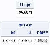
The results of the nonlinear optimization are the same parameter estimates that were obtained by using PROC GENMOD. In addition, the log-likelihood function evaluate at the optimal values is the same as the "full likelihood" value that is reported by PROC GENMOD.

Summary

This article uses nonlinear optimization in PROC IML to reproduce the results of the maximum likelihood estimates for a PROC GENMOD regression model. The article shows how to define the log-likelihood function that is maximized. It also shows that the estimates for the magnitude of the error term is different between the MLE and OLS methods, and that the MLE estimate is smaller. This is the reason that PROC GENMOD and PROC REG obtain different estimates for the same data and model. It also explains why the Parameter Estimates table for PROC GENMOD contains an extra row for the Scale parameter, and why PROC GENMODE displays a note that states, "The scale parameter was estimated by maximum likelihood."

Blogs