Restricted least squares regression in SAS

A data analyst recently asked a question about restricted least square regression in SAS. Recall that a restricted regression puts linear constraints on the coefficients in the model. Examples include forcing a coefficient to be 1 or forcing two coefficients to equal each other. Each of these problems can be solved by using PROC REG in SAS. The analyst's question was, "Why can I use PROC REG to solve a restricted regression problem when the restriction involves EQUALITY constraints, but PROC REG can't solve a regression problem that involves an INEQUALITY constraint?"

This article shows how to use the RESTRICT statement in PROC REG to solve a restricted regression problem that has linear constraints on the parameters. I also use geometry and linear algebra to show that solving an equality-constrained regression problem is mathematically similar to solving an unrestricted least squares system of equations. This explains why PROC REG can solve equality-constrained regression problems. In a future article, I will show how to solve regression problems that involve inequality constraints on the parameters.

The geometry of restricted regression

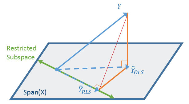
The linear algebra for restricted least squares regression gets messy, but the geometry is easy to picture. A schematic depiction of restricted regression is shown to the right.

Geometrically, ordinary least-squares (OLS) regression is the orthogonal projection of the observed response (Y) onto the column space of the design matrix. (For continuous regressors, this is the span of the X variables, plus an "intercept column.") If you introduce equality constraints among the parameters, you are restricting the solution to a linear subspace of the span (shown in green). But the geometry doesn't change. The restricted least squares (RLS) solution is still a projection of the observed response, but this time onto the restricted subspace.

In terms of linear algebra, the challenge is to write down the projection matrix for the restricted problem. As shown in the diagram, you can obtain the RLS solution in two ways:

Starting from Y: You can directly project the Y vector onto the restricted subspace. The linear algebra for this method is straightforward and is often formulated in terms of Lagrange multipliers.
Starting from the OLS solution: If you already know the OLS solution, you can project that solution vector onto the restricted subspace. Writing down the projection matrix is complicated, so I refer you to the online textbook Practical Econometrics and Data Science by A. Buteikis.

Restricted models and the TEST statement in PROC REG

Let's start with an example, which is based on an example in the online textbook by A. Buteikis. The following SAS DATA step simulates data from a regression model
Y = B0 + B1*X1 + B2*X2 + B3*X3 + B4*X4 + ε
where B3 = B1 and B4 = –2*B2 and ε ~ N(0, 3) is a random error term.

/* Model: Y = B0 + B1*X1 + B2*X2 + B3*X3 + B4*X4
   where B3 = B1 and B4 = -2*B2
*/
data RegSim;
array beta[0:4] (-5, 2, 3, 2, -6);  /* parameter values for regression coefficients */
N = 100;                            /* sample size */
call streaminit(123);
do i = 1 to N;
   x1 = rand("Normal", 5, 2);       /* X1 ~ N(5,2) */
   x2 = rand("Integer", 1, 50);     /* X2 ~ random integer 1:50 */
   x3 = (i-1)*10/(N-1);             /* X3 = sequence: 0 to 10 by 1/N */
   x4 = rand("Normal", 10, 3);      /* X4 ~ N(10, 3) */
   eps = rand("Normal", 0, 3);      /* RMSE = 3 */
   Y = beta[0] + beta[1]*x1 + beta[2]*x2 + beta[3]*x3 + beta[4]*x4 + eps;
   output;
end;
run;

Although there are five parameters in the model (B0-B4), there are only three free parameters because the values of B2 and B4 are determined by the values of B1 and B4, respectively.

If you suspect that a parameter in your model is a known constant or is equal to another parameter, you can use the RESTRICT statement in PROC REG to incorporate that restriction into the model. Before you do, however, it is usually a good idea to perform a statistical test to see if the data supports the model. For this example, you can use the TEST statement in PROC REG to hypothesize that B3 = B1 and B4 = –2*B2. Recall that the syntax for the TEST statement uses the variable names (X1-X4) to represent the coefficients of the variable. The following call to PROC REG carries out this analysis:

proc reg data=RegSim plots=none;
   model Y = x1 - x4;
   test x3 = x1, x4 = -2*x2;
run;

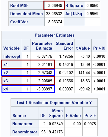
The output shows that the parameter estimates for the simulated data are close to the parameter values used to generate the data. Specifically, the root MSE is close to 3, which is the standard deviation for the error term. The Intercept estimate is close to -5. The coefficients for the X1 and X3 term are each approximately 2. The coefficient for X4 is approximately –2 times the coefficient of X2. The F test for the test of hypotheses has a large p-value, so you should not reject the hypotheses that B3 = B1 and B4 = –2*B2.

The RESTRICT statement in PROC REG

If the hypothesis on the TEST statement fails to reject, then you can use the RESTRICT statement to recompute the parameter estimates subject to the constraints. You could rerun the entire analysis or, if you are running SAS Studio in interactive mode, you can simply submit a RESTRICT statement and PROC REG will compute the new parameter estimates without rereading the data:

   restrict x3 = x1, x4 = -2*x2; /* restricted least squares (RLS) */
   print;
quit;

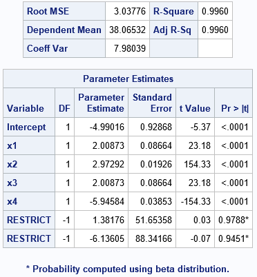
The new parameter estimates enforce the restrictions among the regression coefficients. In the new model, the coefficients for X1 and X3 are exactly equal, and the coefficient for X4 is exactly –2 times the coefficient for X2.

Notice that the ParameterEstimates table is augmented by two rows labeled "RESTRICT". These rows have negative degrees of freedom because they represent constraints. The "Parameter Estimate" column shows the values of the Lagrange multipliers that are used to enforce equality constraints while solving the least squares system. Usually, a data analyst does not care about the actual values in these rows, although the Wikipedia article on Lagrange multipliers discusses ways to interpret the values.

The linear algebra of restricted regression

This section shows the linear algebra behind the restricted least squares solution by using SAS/IML. Recall that the usual way to compute the unrestricted OLS solution is the solve the "normal equations" (X`*X)*b = X`*Y for the parameter estimates, b. Although textbooks often solve this equation by using the inverse of the X`X matrix, it is more efficient to use the SOLVE function in SAS/IML to solve the equation, as follows:

proc iml;
varNames = {x1 x2 x3 x4};
use RegSim;                  /* read the data */
   read all var varNames into X;
   read all var "Y";
close;
X = j(nrow(X), 1, 1) || X;   /* add intercept column to form design matrix */
XpX = X`*X;
 
/* Solve the unrestricted OLS system */
b_ols = solve(XpX, X`*Y);    /* normal equations X`*X * b = X`*Y */
ParamNames = "Intercept" || varNames;
print b_ols[r=ParamNames F=10.5];

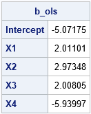
The OLS solution is equal to the first (unrestricted) solution from PROC REG.

If you want to require that the solution satisfies B3 = B1 and B4 = –2*B2, then you can augment the X`X matrix to enforce these constraints. If L*λ = c is the matrix equation for the linear constraints, then the augmented system is
$\begin{pmatrix} X^{\prime}X & L^{\prime} \\ L & 0 \end{pmatrix} \begin{pmatrix} b_{\small\mathrm{RLS}} \\ \lambda \end{pmatrix} = \begin{pmatrix} X^{\prime}Y \\ c \end{pmatrix}$

The following statements solve the augmented system:

/* Direct method: Find b_RLS by solving augmented system */
/* Int X1 X2 X3 X4 */
L = {0  1  0 -1  0,     /*    X1 - X3 = 0 */
     0  0 -2  0 -1};    /* -2*X2 - X4 = 0 */
c = {0, 0};
 
zero = j(nrow(L), nrow(L), 0);
A = (XpX || L`   ) //
    (L   || zero );
z = X`*Y // c;
b_rls = solve(A, z);
rNames = ParamNames||{'Lambda1' 'Lambda2'};
print b_rls[r=rNames F=10.5];

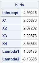
The parameter estimates are the same as are produced by using PROC REG. You can usually ignore the last two rows, which are the values of the Lagrange multipliers that enforce the constraints.

By slogging through some complicated linear algebra, you can also obtain the restricted least squares solution from the OLS solution and the constraint matrix (L). The following equations use the formulas in the online textbook by A. Buteikis to compute the restricted solution:

/* Adjust the OLS solution to obtain the RLS solution.
   b_RLS = b_OLS - b_adjustment
   Follows
   http://web.vu.lt/mif/a.buteikis/wp-content/uploads/PE_Book/4-4-Multiple-RLS.html
*/
RA_1 = solve(XpX, L`);
RA_3 = solve(L*RA_1, L*b_ols - c);
b_adj = RA_1 * RA_3;
b_rls = b_ols - b_adj;
print b_rls[r=ParamNames F=10.5];

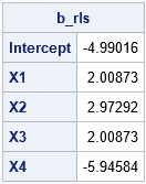
This answer agrees with the previous answer but does not compute the Lagrange multipliers. Instead, it computes the RLS solution as the projection of the OLS solution onto the restricted linear subspace.

Summary

This article shows how to use the RESTRICT statement in PROC REG to solve a restricted regression problem that involves linear constraints on the parameters. Solving an equality-constrained regression problem is very similar to solving an unrestricted least squares system of equations. Geometrically, they are both projections onto a linear subspace. Algebraically, you can solve the restricted problem directly or as the projection of the OLS solution.

Although changing one of the equality constraints into an INEQUALITY seems like a minor change, it means that the restricted region is no longer a linear subspace. Ordinary least squares can no longer solve the problem because the solution might not be an orthogonal projection. The next article discusses ways to solve problems where the regression coefficients are related by linear inequalities.

Blogs