An early method for robust regression was iteratively reweighted least-squares regression (Huber, 1964). This is an iterative procedure in which each observation is assigned a weight. Initially, all weights are 1. The method fits a least-squares model to the weighted data and uses the size of the residuals to determine a new set of weights for each observation. In most implementations, observations that have large residuals are downweighted (assigned weights less than 1) whereas observations with small residuals are given weights close to 1. By iterating the reweighting and fitting steps, the method converges to a regression that de-emphasizes observations whose residuals are much bigger than the others.

This form of robust regression is also called M estimation. The "M" signifies that the method is similar to Maximum likelihood estimation. The method tries to minimize a function of the weighted residuals. This method is not robust to high-leverage points because they have a disproportionate influence on the initial fit, which often means they have small residuals and are never downweighted.

The results of the regression depend on the function that you use to weight the residuals. The ROBUSTREG procedure in SAS supports 10 different "weighting functions." Some of these assign a zero weight to observations that have large residuals, which essentially excludes that observation from the fit. Others use a geometric or exponentially decaying function to assign small (but nonzero) weights to large residual values. This article visualizes the 10 weighting functions that are available in SAS software for performing M estimation in the ROBUSTREG procedure. You can use the WEIGHTFUNCTION= suboption to the METHOD=M option on the PROC ROBUSTREG statement to choose a weighting function.

See the documentation of the ROBUSTREG procedure for the formulas and default parameter values for the 10 weighting functions. The residuals are standardized by using a robust estimate of scale. In the rest of this article, "the residual" actually refers to a standardized residual, not the raw residual. The plots of the weighting functions are shown on the interval[-6, 6] and show how functions assign weights based on the magnitude of the standardized residuals.

Differentiable weighting functions

If you are using iteratively reweighted least squares to compute the estimates, it doesn't matter whether the weighting functions are differentiable. However, if you want to use optimization methods to solve for the parameter estimates, many popular optimization algorithms work best when the objective function is differentiable. The objective function is often related to a sum that involves the weighted residuals, so let's first look at weighting functions that are differentiable. The following four functions are differentiable transformations that assign weights to observations based on the size of the standardized residual.

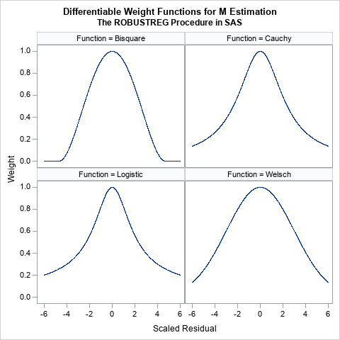
These functions all look similar. They are all symmetric functions and look like the quadratic function 1 – a r² close to r = 0. However, the functions differ in the rate at which they decrease away from r = 0:

• The bisquare function (also called the Tukey function) is a quartic function on the range [-c, c] and equals 0 outside that interval. This is the default weight function for M estimation in PROC ROBUSTREG. The function is chosen so that the derivative at ±c is 0, and thus the function is differentiable. An observation is excluded from the computation if the magnitude of the standardized residual exceeds c. By default, c=4.685.
• The Cauchy and Logistic functions are smooth functions that decrease exponentially. If you use these functions, the weight for an observation is never 0, but the weight falls off rapidly as the magnitude of r increases.
• The Welsch function is a rescaled Gaussian function. The weight for an observation is never 0, but the weight falls off rapidly (like exp(-a r²)) as the magnitude of r increases.

Nondifferentiable weighting functions

The following six functions are not differentiable at one or more points.

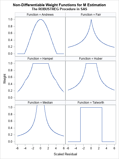
• The Andrews function is the function c*sin(r/c)/r within the interval [-c π, c π] and 0 outside. It is similar to the bisquare function (see the previous section) but is not differentiable at ±c π.
• The Fair and Median functions are similar. The assign a weight that is asymptotically proportional to 1/|r|. Use the Fair function if you want to downweight observations according to the inverse magnitude of their residual value. Do not use the Median function, which assigns huge weights to observations with small residuals.
• The Hampel, Huber, and Talworth functions are similar because they all assign unit weight to residuals that are small in magnitude. The Talworth function is the most Draconian weight function: it assigns each observation a weight of 1 or 0, depending on whether the magnitude of the residual exceeds some threshold. The Hampel and Huber functions assign a weight of 1 for small residuals, then assign weights in a decreasing manner. If you use the default parameter values for the Hampel function, the weights are exactly 0 outside of the interval [-8, 8].

When I use M estimation, I typically use one of the following three functions:

• The bisquare function, which excludes observations whose residuals have a magnitude greater than 4.685.
• The Welsch function, which gently downweights large residuals.
• The Huber function, which assigns 1 for the weight of small residuals and assigns weights to larger residuals that are proportional to the inverse magnitude.

Summary

M estimation is a robust regression technique that assigns weights to each observation. The idea is to assign small (or even zero) weights to observations that have large residuals and weights that are close to unity for residuals that are small. (In practice, the algorithm uses standardize residuals to assign weights.) There are many ways to assign weights, and SAS provides 10 different weighting functions. This article visualizes the weighting functions. The results of the regression depend on the function that you use to weight the residuals.

Appendix: SAS program to visualize the weighting functions in PROC ROBUSTREG

I used SAS/IML to define the weighting functions because the language supports default arguments for functions, whereas PROC FCMP does not. Each function evaluates a vector of input values (x) and returns a vector of values for the weighting function. The default parameter values are specified by using the ARG=value notation in the function signature. If you do not specify the optional parameter, the default value is used.

The following statements produce a 2 x 2 panel of graphs that shows the shapes of the bisquare, Cauchy, logistic, and Welsch functions:

/***********************************/
/* Differentiable weight functions */
/* Assume x is a column vector     */
/***********************************/
 
proc iml;
/* The derivative of Bisquare is f'(x)=4x(x^2-c^2)/c^4, so f'( +/-c )= 0 
   However, second derivative is f''(x) = 4(3x^2-c^2)/c^4, so f''(c) ^= 0 
*/
start Bisquare(x, c=4.685);   /* Tukey's function */
   w = j(nrow(x), 1, 0);   /* initialize output */
   idx = loc( abs(x) <= c );
   if ncol(idx)>0 then do;
      y = x[idx]/c;
      w[idx] = (1 - y##2)##2;
   end;
   return ( w );
finish;
 
start Cauchy(x, c=2.385);
   w = 1 / (1 + (abs(x)/c)##2);
   return ( w );
finish;
 
start Logistic(x, c=1.205);
   w = j(nrow(x), 1, 1);   /* initialize output */
   idx = loc( abs(x) > constant('maceps') ); /* lim x->0 f(x) = 1 */
   if ncol(idx)>0 then do;
      y = x[idx]/c;
      w[idx] = tanh(y) / y;
   end;
   return ( w );
finish;
 
start Welsch(x, c=2.985);
   w = exp( -(x/c)##2 / 2 );
   return ( w );
finish;
 
x = T(do(-6, 6, 0.005));
Function = j(nrow(x), 1, BlankStr(12));
 
create WtFuncs var {'Function' 'x' 'y'};
y = Bisquare(x);  Function[,] = "Bisquare"; append;
y = Cauchy(x);    Function[,] = "Cauchy";   append;
y = Logistic(x);  Function[,] = "Logistic"; append;
y = Welsch(x);    Function[,] = "Welsch";   append;
close;
 
quit;
 
ods graphics/ width=480px height=480px;
title "Differentiable Weight Functions for M Estimation";
title2 "The ROBUSTREG Procedure in SAS";
proc sgpanel data=WtFuncs;
   label x = "Scaled Residual" y="Weight";
   panelby Function / columns=2;
   series x=x y=y;
run;

The following statements produce a 3 x 2 panel of graphs that shows the shapes of the Andrews, Fair, Hampel, Huber, median, and Talworth functions:

/*******************************/
/* Non-smooth weight functions */
/* Assume x is a column vector */
/*******************************/
proc iml;
 
start Andrews(x, c=1.339);
   w = j(nrow(x), 1, 0);   /* initialize output */
   idx = loc( abs(x) <= constant('pi')*c );
   if ncol(idx)>0 then do;
      y = x[idx]/c;
      w[idx] = sin(y) / y;
   end;
   return ( w );
finish;
 
start Fair(x, c=1.4);
   w = 1 / (1 + abs(x)/c);
   return ( w );
finish;
 
start Hampel(x, a=2, b=4, c=8);
   w = j(nrow(x), 1, 0);   /* initialize output */
   idx = loc( abs(x) <= a );
   if ncol(idx)>0 then
     w[idx] = 1;
   idx = loc( a < abs(x) & abs(x) <= b );
   if ncol(idx)>0 then
     w[idx] = a / abs(x[idx]);
   idx = loc( b < abs(x) & abs(x) <= c );
   if ncol(idx)>0 then
     w[idx] = (a / abs(x[idx])) # (c - abs(x[idx])) / (c-b);
   return ( w );
finish;
 
start Huber(x, c=1.345);
   w = j(nrow(x), 1, 1);   /* initialize output */
   idx = loc( abs(x) >= c );
   if ncol(idx)>0 then do;
      w[idx] = c / abs(x[idx]);
   end;
   return ( w );
finish;
 
start MedianWt(x, c=0.01);
   w = j(nrow(x), 1, 1/c);   /* initialize output */
   idx = loc( x ^= c );
   if ncol(idx)>0 then do;
      w[idx] = 1 / abs(x[idx]);
   end;
   return ( w );
finish;
 
start Talworth(x, c=2.795);
   w = j(nrow(x), 1, 0);   /* initialize output */
   idx = loc( abs(x) < c );
   if ncol(idx)>0 then do;
      w[idx] = 1;
   end;
   return ( w );
finish;
 
x = T(do(-6, 6, 0.01));
Function = j(nrow(x), 1, BlankStr(12));
create WtFuncs var {'Function' 'x' 'y'};
 
y = Andrews(x);  Function[,] = "Andrews"; append;
y = Fair(x);     Function[,] = "Fair";    append;
y = Hampel(x);   Function[,] = "Hampel";  append;
y = Huber(x);    Function[,] = "Huber";   append;
y = MedianWt(x); Function[,] = "Median";  append;
y = Talworth(x); Function[,] = "Talworth";append;
close;
quit;
 
ods graphics/ width=480px height=640px;
title "Non-Differentiable Weight Functions for M Estimation";
title2 "The ROBUSTREG Procedure in SAS";
proc sgpanel data=WtFuncs;
   label x = "Scaled Residual" y="Weight";
   panelby Function / columns=2;
   series x=x y=y;
   rowaxis max=1;
run;