Create a probability distribution from almost any positive function

There are dozens of common probability distributions for a continuous univariate random variable. Familiar examples include the normal, exponential, uniform, gamma, and beta distributions. Where did these distributions come from? Well, some mathematician needed a model for a stochastic process and wrote down the equation for the distribution, typically by specifying the probability density function.

You might think that these mathematicians were very clever (they were!), but it isn't that difficult to create a new univariate continuous distribution that has never been studied before. You can start with almost any positive (actually, nonnegative is okay) function such as a polynomial, exponential, or trigonometric function on some domain, D ⊆ R. You must normalize the function so that it has unit area over D. In advanced courses such as measure theory, you learn that there are certain technical restrictions on the function and its domain, but I will ignore those technical details in this article.

How to create a probability distribution

Here are the steps you can take to create a new probability distribution:

Choose any nonnegative, piecewise continuous, integrable function, w, on a finite or infinite domain, D ⊆ R.
Nonnegative means that w(x) ≥ 0 for all x in D. If necessary, extend w to the whole real line by defining it to be identically 0 outside of D.
Integrable means that the integral of the function on D is finite. Let A = ∫_D w(x) dx be the value of the integral.
Define f(x) = w(x) / A for all values of x. The function f is a probability density function (PDF) because f ≥ 0 and ∫_D f(x) dx = 1.

From the density function, you can derive the cumulative distribution (CDF), quantile function, and random variates. So—voila!—you have defined the PDF for a probability distribution!

Let's illustrate these steps with two familiar examples:

The exponential function w(x) = exp(-βx) is positive on the interval D = [0, ∞). The integral on D is 1/β. Therefore, the function f(x) = β exp(-βx) is a probability density on D. Extend the density to the whole line by defining f(x)=0 for x < 0.
The bell-shaped function w(x) = exp(-x²/2) is positive on entire line D = (-∞, ∞). The integral on D is sqrt(2π). Therefore, the function f(x) = (1/sqrt(2π)) exp(-x²/2) is a probability density on the real line.

Create a new probability distribution

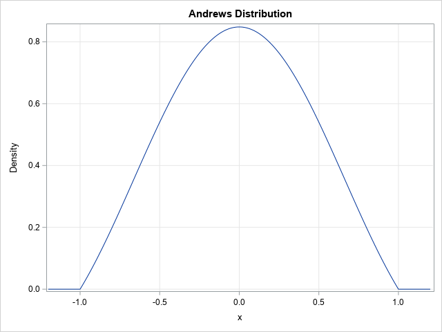
Let's create a new probability distribution that has never been studied (as far as I know). In a previous article, I discussed a series of 10 weight functions that are used for robust regression models. Of these, 9 are integrable (avoid the "median" weight function!). Let's make a probability distribution from the Andrews function, which is defined as w(x) = sin(π x)/(π x) on the interval [-1, 1]. The Andrews function is nonnegative on [-1, 1]. The integral does not have a closed-form solution in terms of elementary functions, but the numerical value is S=1.1789797 (see the Appendix for this computation). Therefore, our new "Andrews distribution" has a probability density equal to f(x) = (1/S) sin(π x)/(π x) on the interval [-1, 1] and 0 otherwise. The graph of the density function is shown below.

From the PDF to all other distribution functions

In theory, you can obtain all other distribution functions from the PDF:

The cumulative distribution function at any value x in [-1,1] is obtained by the area under the density curve: F(x) = ∫_-1^x f(t) dt.
The quantile function is inverse CDF, which requires finding the root F(x) = q for a given quantile q in (0, 1).
You can generate random variates from the distribution by using the inverse CDF method.

In practice, I would probably not compute the CDF and the quantile function dynamically. Rather, I would tabulate the CDF and quantile function on a fine grid of values and then use linear interpolation between the tabulated values as needed. As for generating random variates, I would probably not use the inverse CDF method because it is too inefficient. Instead, I would use an acceptance-rejection method to simulate random variates.

Summary

In summary, you can create a new probability distribution from any integrable positive function, w. The trick is to compute the integral of the function (A) over a specified domain and then define a probability density as f(x) = w(x) / A. From the density function, you can obtain all the other important functions for studying the distribution. The next blog post shows how to use an acceptance-rejection method to generate random variates for the Andrews distribution.

Appendix: Deriving and graphing the Andrews distribution

The following SAS IML program uses the QUAD function to compute the area under the density curve for the Andrews distribution:

proc iml;
/* Andrews weight function with c = 1/pi */
start Andrews(x);
   if x=0 then return(1);
   pi = constant('pi');
   return( sin(pi*x) / (pi*x) );
finish;
 
call quad(S, 'Andrews', {-1, 1});  /* integral on [-1, 1] */
print S;
QUIT;

After you know the standardizing factor, you can graph the probability density function:

data Andrews;
S = 1.1789797;
pi = constant('pi');
xMin = -1.2; xMax = 1.2; dx = 0.01;
do x = xMin to xMax by dx;
   /* Andrews distribution = scaled version of Andrews weight function */
   if abs(x) <= 1 then do;
      if x=0 then f = 1/S;
      else f = sin(pi*x) / (pi*x) / S;
   end;
   else f = 0;
   output;
end;
keep x f;
run;
 
title "Probability Density for Andrews Distribution";
proc sgplot data=Andrews;
   series x=x y=f;
   yaxis grid label="Density";
   xaxis grid;
run;

The graph is shown earlier in this article.

Blogs