In my previous post, I showed how to approximate a cumulative density function (CDF) by evaluating only the probability density function. The technique uses the trapezoidal rule of integration to approximate the CDF from the PDF.

For common probability distributions, you can use the CDF function in Base SAS to evaluate the cumulative distributions. The technique from my previous post becomes relevant if you need to compute the CDF of a distribution that is not built into SAS.

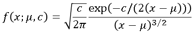
A recent question on a discussion forum was "How can I plot the PDF and CDF for [an unsupported]distribution?" It turns out that the distribution from the discussion forum has an analytical expression for the CDF, so I will use the Lévy distribution for this article. The density of the Lévy distribution is given by the following formula:

Evaluating a custom PDF in SAS

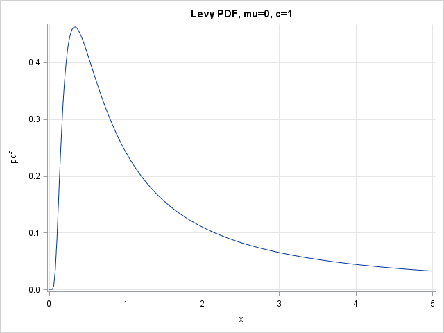
When evaluating any function in SAS, you need to make sure that you understand the domain of the function. For the Lévy distribution, the support is the semi-infinite interval [μ, ∞). The location parameter μ determines the left-hand endpoint for the support of the distribution. The scale parameter c must be a positive value. The limit as x → μ⁺ is 0. The following SAS/IML module evaluates the Lévy density function. The function is vectorized so that it returns a vector of densities if you call it with a vector of x values. The implementation sets default parameter values of μ=0 and c=1.

proc iml;
start LevyPDF(x, mu=0, c=1);
   pi = constant("pi");
   f = j(nrow(x), ncol(x), 0);         /* any values outside support are 0 */
   idx = loc(x>mu);                    /* find valid values of x */
   if ncol(idx)>0 then do;             /* evaluate density for valid values */
      v = x[idx];         
      f[idx] = sqrt(c/(2*pi)) # exp(-c/(2*(v-mu))) /(v-mu)##1.5; 
   end;
   return( f );
finish;
 
/* plot PDF on [0, 5] */
x = do(0,5,0.02);
pdf = LevyPDF(x);
title "Levy PDF, mu=0, c=1";
call Series(x, pdf) grid={x y};

Evaluating a custom CDF in SAS: The quick-and-dirty way

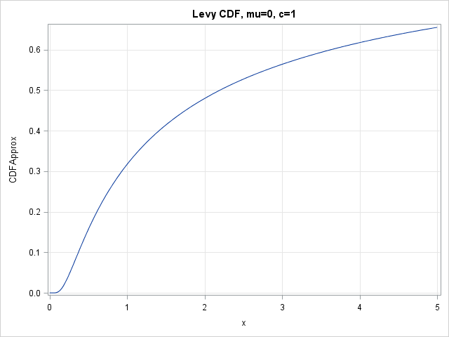
As shown in my previous post, you can approximate a cumulative density function (CDF) by using the trapezoidal rule to add up the area under the PDF. The following statements implement this approximation. The approximation is accurate provided that the distance between adjacent x values is small, especially when the second derivative of the PDF is large.

start CumTrapIntegral(x,y);      /* cumulative sums of trapezoidal areas */
   N = nrow(colvec(x));
   dx    =   x[2:N] - x[1:N-1];
   meanY = ( y[2:N] + y[1:N-1] )/2;
   return( 0 // cusum(dx # meanY) );
finish;
 
CDFApprox = CumTrapIntegral(x, pdf);   
title "Levy CDF, mu=0, c=1";
call Series(x, CDFApprox) yvalues=do(0,0.7,0.1) grid={x y};

Evaluating a custom CDF in SAS: The slow-and-steady way

Although the trapezoidal approximation of the CDF is very fast to compute, sometimes slow and steady wins the race. If you want to evaluate the CDF as accurately as possible, or you only need the CDF at a few locations, you can use the QUAD subroutine to numerically integrate the PDF.

To use the QUAD subroutine, the integrand must be a function of a single variable (x). Any parameters (such as μ and c) must be specified by using a GLOBAL clause. The following statements define a function named _Func that calls the LevyPDF function with the value of the global parameters g_mu and g_c. From the plot of the CDF function, it looks like the median of the distribution is approximately at x=2.2. The following statements evaluate the integral of the Lévy PDF on the interval [0, 2.2]. The integral is approximately 0.5.

start _Func(x) global(g_mu, g_c);
   return( LevyPDF(x, g_mu, g_c) );
finish;
 
/* looks like median is about x=2.2 */
g_mu=0; g_c=1;
call quad(result, "_Func", {0 2.2});
print result;

The call to the QUAD subroutine gave the expected answer. Therefore you can create a function that calls the QUAD subroutine many times to evaluate the Lévy cumulative distribution at a vector of values:

start LevyCDF(x, mu=0, c=1) global(g_mu, g_c);
   cdf = j(nrow(x), ncol(x), 0);             /* allocate result */
   N = nrow(x)*ncol(x);
   g_mu=mu; g_c=c;
   do i = 1 to N;                            /* for each x value */
      call quad(result, "_Func", 0 || x[i]); /* compute integral on [0,x] */
      cdf[i] = result;
   end;
   return(cdf);
finish;
 
CDF = LevyCDF(x);
title "Levy CDF, mu=0, c=1";
call Series(x, CDF) yvalues=do(0,0.7,0.1) grid={x y};

The graph is visually indistinguishable from the previous CDF graph and is not shown. The CDF curve computed by calling the LevyCDF function is within 2e-5 of the approximate CDF curve. However, the approximate curve is computed almost instantaneously, whereas the curve that evaluates integrals requires a noticeable fraction of a second.

In summary, if you implement a custom probability distribution in SAS, try to write the PDF function so that it is vectorized. Pay attention to special points in the domain (such as 0) that might require special handling. From the PDF, you can create a CDF function. You can use the CumTrapIntegral function to evaluate an approximate CDF from values of the PDF, or you can use the QUAD function to create a computationally expensive (but more accurate) function that integrates the PDF.