The generalized gamma distribution

A SAS customer wanted to compute the cumulative distribution function (CDF) of the generalized gamma distribution. For any continuous distribution, the CDF is the integral of the probability density function (PDF), which usually has an explicit formula. Accordingly, he wanted to compute the CDF by using the QUAD function in PROC IML to integrate the PDF.

I have previously shown how to integrate the PDF to obtain the CDF. I have also shown how to use the trapezoid rule of numerical integration to obtain the entire CDF curve from a curve of the PDF. But before I sent him those links, I looked closer at the distribution that he wanted to compute. It turns out that you don't have to perform an integral to get the CDF of the generalized gamma distribution.

What is the generalized gamma distribution

I was not familiar with the generalized gamma distribution, so I looked at an article on Wikipedia. The original formulation is due to Stacy, E. (1962), "A Generalization of the Gamma Distribution." The distribution is "generalized" in the sense that it contains many other familiar distributions for certain parameter values, including the gamma, chi-square, exponential, half-normal, and Weibull distributions.

The following definition is from Wikipedia, but I changed the notation for the incomplete gamma function to agree with my previous article. The generalized gamma has three parameters: a>0, d>0, and p>0. For non-negative x, the probability density function of the generalized gamma is
$f(x;a,d,p)=(p/a^{d})x^{d-1}e^{-(x/a)^{p}} / \,\Gamma (d/p)$
where $\Gamma(\cdot)$ denotes the complete gamma function.

The cumulative distribution function is
$F(x;a,d,p)=\gamma ((x/a)^{p}, d/p) / \,\Gamma (d/p)$ ,
where $\gamma (\cdot )$ denotes the lower incomplete gamma function.

Compute the generalized gamma distribution in SAS

Evaluating the PDF is usually easy because it has an explicit formula. It is the CDF that requires thought and effort. In this case, however, the CDF is given in terms of the lower incomplete gamma function, and I recently showed how to compute the lower incomplete gamma function in SAS. As a rule of thumb, if a distribution has 'gamma' as part of its name, you might be able to use this trick to evaluate the CDF.

In my previous article, I showed that the lower incomplete gamma function is nothing more than the "unstandardized" CDF of the gamma distribution, as represented by this SAS macro:

%macro LowerIncGamma(x, alpha); /* lower incomplete gamma function */
   (Gamma(&alpha) * CDF('Gamma', &x, &alpha))
%mend;

But the formula for the CDF of the generalized gamma distribution divides by the complete gamma function, which just leaves the call to the CDF function. Instead of the parameter x, you use (x/a)^p. For the parameter α, you substitute α=d/p. This means that you can compute the CDF for the generalized gamma distribution by using the CDF('GAMMA') function in SAS. The following SAS DATA step evaluates the PDF and CDF for five combinations of the a, d, and p parameters. These are the same parameter values that are used in the Wikipedia article.

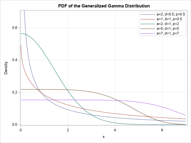
data GenGamma;
label PDF = "Density" CDF = "Cumulative Probability";
array _a[5] _temporary_ (2,   1,   2, 5, 7);
array _d[5] _temporary_ (0.5, 1,   1, 1, 1);
array _p[5] _temporary_ (0.5, 0.5, 2, 5, 7);
do i = 1 to dim(_a);
   a = _a[i]; d = _d[i]; p = _p[i];
   params = cats('a=',a,', d=',d,', p=',p);
   do x = 0.0001, 0.001, 0.01 to 7 by 0.01;
      PDF = (p/a**d) * x**(d-1) * exp(-(x/a)**p) / Gamma(d/p);
      CDF = CDF('Gamma', (x/a)**p, d/p);
      output;
   end;
end;
run;

The following call to PROC SGPLOT creates a graph of the PDF for the five sets of parameter values:

title "PDF of the Generalized Gamma Distribution";
proc sgplot data=GenGamma;
   series x=x y=PDF / group=params;
   yaxis max = 0.7 grid;
   xaxis grid;
   keylegend / location=inside position=NE across=1 title="" opaque;
run;

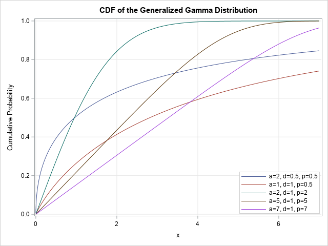
The PDF curves are shown in the graph in the previous section. You can use almost the same statements to create a graph of the five CDF functions:

title "CDF of the Generalized Gamma Distribution";
proc sgplot data=GenGamma;
   series x=x y=CDF / group=params;
   yaxis grid;
   xaxis grid;
   keylegend / location=inside position=SE across=1 title="" opaque;
run;

Quantiles of the generalized gamma distribution

Although the SAS programmer did not request the quantile function for the generalized gamma distribution, it can be evaluated by using the QUANTILE('GAMMA") function in SAS. The details are in the Wikipedia article. For completeness, the following DATA step computes the quantiles. The graph is not shown, since it is the same as the graph of the cumulative distribution, but with the axes interchanged.

data GenGammaQuantile;
label prob = "Cumulative Probability" q = "Quantile";
array _a[5] _temporary_ (2,   1,   2, 5, 7);
array _d[5] _temporary_ (0.5, 1,   1, 1, 1);
array _p[5] _temporary_ (0.5, 0.5, 2, 5, 7);
do i = 1 to dim(_a);
   a = _a[i]; d = _d[i]; p = _p[i];
   params = cats('a=',a,', d=',d,', p=',p);
   do prob = 0.001, 0.01 to 0.99 by 0.01;
      y = quantile("Gamma", prob, d/p);
      q = a * y**(1/p);
      output;
   end;
end;
run;
 
title "Quantiles of the Generalized Gamma Distribution";
proc sgplot data=GenGammaQuantile;
   series x=prob y=q / group=params;
   yaxis grid max=7;
   xaxis grid;
   keylegend / location=inside position=NW across=1 title="" opaque;
run;

Summary

Although you can integrate the PDF to obtain the CDF for a continuous probability distribution, sometimes it is possible to evaluate the CDF in an easier way. In the case of the generalized gamma distribution, the CDF can be evaluated by using the CDF of the ordinary gamma distribution. You just need to be clever about how to pass in the parameter values.

Federico Bonofiglio on July 25, 2024 12:13 pm

Hi Rick, this was a great post which prompted me to do some extra research because I needed to manually reproduce quantiles from the PROC LIFEREG output with dist = Gamma (that is GENGAMMA). Your trick was not immediately applicable because LIFEREG uses a different parametrization (see supported distributions) making regression optimization more stable. Therefore, the missing step was to map the LIFEREG parametrization to the one you use above except that k = d/p (a slightly different reparametrization, see Lawless https://www.jstor.org/stable/1268326). I show this for the quantile but reproducing the density should be straightforward using the mapping in the res_gamma data step. Note that in the documentation for predicting values (https://go.documentation.sas.com/doc/en/pgmsascdc/9.4_3.4/statug/statug_lifereg_details12.htm) it is said that a numerical step for the quantile function is used. Instead, what do you see below could be an handy closed-form alternative.
I hope this might be of any interest. Best ;)

/*using data from SAS LIFEREG documentation*/

title 'Motorette Failures With Operating Temperature as a Covariate';
data motors;
input time censor temp @@;
if _N_=1 then
do;
temp=130;
time=.;
control=1;
z=1000/(273.2+temp);
output;
temp=150;
time=.;
control=1;
z=1000/(273.2+temp);
output;
end;
if temp>150;
control=0;
z=1000/(273.2+temp);
output;
datalines;
8064 0 150 8064 0 150 8064 0 150 8064 0 150 8064 0 150
8064 0 150 8064 0 150 8064 0 150 8064 0 150 8064 0 150
1764 1 170 2772 1 170 3444 1 170 3542 1 170 3780 1 170
4860 1 170 5196 1 170 5448 0 170 5448 0 170 5448 0 170
408 1 190 408 1 190 1344 1 190 1344 1 190 1440 1 190
1680 0 190 1680 0 190 1680 0 190 1680 0 190 1680 0 190
408 1 220 408 1 220 504 1 220 504 1 220 504 1 220
528 0 220 528 0 220 528 0 220 528 0 220 528 0 220
;

run;

/* RUN REGRESSION
*/

proc lifereg data=motors;
model time*censor(0)=z /dist=gamma;
output out=out_gamma predicted=pred_ xbeta=xb_;
ods output ParameterEstimates=parm_gamma;
run;

/*analytical calculation of GENGAMMA quantile that uses PROC LIFEREG parametrization is broken down into three steps:

1) obtain coefficients from PROC LIFEREG (stable parametrization https://go.documentation.sas.com/doc/en/pgmsascdc/9.4_3.4/statug/statug_lifereg_details04.htm)
2) map obtained coefficients to original GENGAMMA parametrization
3) map original gengamma parametrization to classical Gamma parameters based on https://blogs.sas.com/content/iml/2021/03/15/generalized-gamma-distribution.html

NOTE: calculations in step 2, 3 must be performed by hand, result are below
*/

/* extract estimates based on SAS documentation stable parametrization */

data _null_;
set work.parm_gamma;
where Parameter eq "Scale";
call symput('sigma', Estimate);
run;
%put &=sigma;

data _null_;
set work.parm_gamma;
where Parameter eq "Shape";
call symput('Q', Estimate);
run;
%put &=Q;

/*map stable parametrization to parameters of original GENGAMMA distribution
and to PROC LIFEREG quantile using relation to GAMMA distribution (step 2, 3).
Make use of Xbeta from out dataset
*/

data res_gamma;
set work.out_gamma;
k = 1/(&Q.*&Q.);
p = &Q./&sigma.;
log_a = xb_ - log(k)/p;
log_up = log(quantile("GAMMA", 0.5, k)); /* use percentile = 0.5 as by default in lifereg*/
pred_reproduce = exp(log_a + (1/p)*log_up); /*compare to pred_*/
run;

proc print data=res_gamma;

2 Comments

Federico Bonofiglio on July 25, 2024 12:13 pm

Hi Rick, this was a great post which prompted me to do some extra research because I needed to manually reproduce quantiles from the PROC LIFEREG output with dist = Gamma (that is GENGAMMA). Your trick was not immediately applicable because LIFEREG uses a different parametrization (see supported distributions) making regression optimization more stable. Therefore, the missing step was to map the LIFEREG parametrization to the one you use above except that k = d/p (a slightly different reparametrization, see Lawless https://www.jstor.org/stable/1268326). I show this for the quantile but reproducing the density should be straightforward using the mapping in the res_gamma data step. Note that in the documentation for predicting values (https://go.documentation.sas.com/doc/en/pgmsascdc/9.4_3.4/statug/statug_lifereg_details12.htm) it is said that a numerical step for the quantile function is used. Instead, what do you see below could be an handy closed-form alternative.
I hope this might be of any interest. Best ;)

/*using data from SAS LIFEREG documentation*/

title 'Motorette Failures With Operating Temperature as a Covariate';
data motors;
input time censor temp @@;
if _N_=1 then
do;
temp=130;
time=.;
control=1;
z=1000/(273.2+temp);
output;
temp=150;
time=.;
control=1;
z=1000/(273.2+temp);
output;
end;
if temp>150;
control=0;
z=1000/(273.2+temp);
output;
datalines;
8064 0 150 8064 0 150 8064 0 150 8064 0 150 8064 0 150
8064 0 150 8064 0 150 8064 0 150 8064 0 150 8064 0 150
1764 1 170 2772 1 170 3444 1 170 3542 1 170 3780 1 170
4860 1 170 5196 1 170 5448 0 170 5448 0 170 5448 0 170
408 1 190 408 1 190 1344 1 190 1344 1 190 1440 1 190
1680 0 190 1680 0 190 1680 0 190 1680 0 190 1680 0 190
408 1 220 408 1 220 504 1 220 504 1 220 504 1 220
528 0 220 528 0 220 528 0 220 528 0 220 528 0 220
;

run;

/* RUN REGRESSION
*/

proc lifereg data=motors;
model time*censor(0)=z /dist=gamma;
output out=out_gamma predicted=pred_ xbeta=xb_;
ods output ParameterEstimates=parm_gamma;
run;

/*analytical calculation of GENGAMMA quantile that uses PROC LIFEREG parametrization is broken down into three steps:

1) obtain coefficients from PROC LIFEREG (stable parametrization https://go.documentation.sas.com/doc/en/pgmsascdc/9.4_3.4/statug/statug_lifereg_details04.htm)
2) map obtained coefficients to original GENGAMMA parametrization
3) map original gengamma parametrization to classical Gamma parameters based on https://blogs.sas.com/content/iml/2021/03/15/generalized-gamma-distribution.html

NOTE: calculations in step 2, 3 must be performed by hand, result are below
*/

/* extract estimates based on SAS documentation stable parametrization */

data _null_;
set work.parm_gamma;
where Parameter eq "Scale";
call symput('sigma', Estimate);
run;
%put &=sigma;

data _null_;
set work.parm_gamma;
where Parameter eq "Shape";
call symput('Q', Estimate);
run;
%put &=Q;

/*map stable parametrization to parameters of original GENGAMMA distribution
and to PROC LIFEREG quantile using relation to GAMMA distribution (step 2, 3).
Make use of Xbeta from out dataset
*/

data res_gamma;
set work.out_gamma;
k = 1/(&Q.*&Q.);
p = &Q./&sigma.;
log_a = xb_ - log(k)/p;
log_up = log(quantile("GAMMA", 0.5, k)); /* use percentile = 0.5 as by default in lifereg*/
pred_reproduce = exp(log_a + (1/p)*log_up); /*compare to pred_*/
run;

proc print data=res_gamma;

- Rick Wicklin on July 25, 2024 2:01 pm
  
  Thanks for writing. For more information about different parameterizations encountered in regression procedures, see "Interpret estimates for a Weibull regression model in SAS," which contains a link to some helpful SAS Usage Notes, such as Usage Note 24166. If you scroll down to the "Gamma" section of that note, you will find links to additional Usage Notes.

Blogs