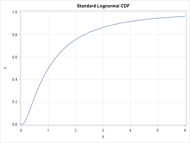
Evaluating a cumulative distribution function (CDF) can be an expensive operation. Each time you evaluate the CDF for a continuous probability distribution, the software has to perform a numerical integration. (Recall that the CDF at a point x is the integral under the probability density function (PDF) where x is the upper limit of integration. I am assuming that the PDF does not have a closed-form antiderivative.) For example, the following statements compute and graph the CDF for the standard lognormal distribution at 121 points in the domain [0,6]. To create the graph, the software has to compute 121 numerical integrations.

proc iml;
x = do(0, 6, 0.05);
CDF = cdf("Lognormal", x);
title "Standard Lognormal CDF";
call series(x, CDF) grid={x y};

An integral is an accumulation of slices

In contrast, evaluating the PDF is relatively cheap: you only need to evaluate the density function at a series of points. No integrals reqired. This suggests a clever little approximation: Instead of calling the CDF function many times, call the PDF function and use the cumulative sum function (CUSUM) to add together the areas of many slices of the density. For example, it is simple to modify the trapezoidal rule of integration to return a cumulative sum of the trapezoidal areas that approximate the area under a curve, as follows:

start CumTrapIntegral(x,y);
   N = nrow(colvec(x));
   dx    =   x[2:N] - x[1:N-1];
   meanY = ( y[2:N] + y[1:N-1] )/2;
   return( 0 // cusum(dx # meanY) );
finish;

With this function you can approximate the (expensive) CDF by using a series of (cheap) PDF evaluations, as follows:

pdf = pdf("Lognormal", x);             /* evaluate PDF */
CDFApprox = CumTrapIntegral(x, pdf);   /* cumulative sums of trapezoidal areas */

How good is the approximation to the CDF? You can plot the difference between the values that were computed by the CDF function and the values that were computed by using the trapeoidal areas:

Difference = CDF - CDFApprox`;
title "Difference between Lognormal CDF and Aproximate CDF";
call Series(x, Difference) grid={x y};

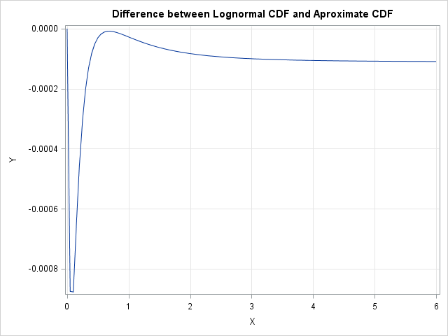
The graph shows that for the lognormal distribution evaluated on [0,6], the approximate CDF differs by less than 0.001. For most values of x, CDF(x) differs from the cumulative trapezoidal approximation by less than 0.0001. This result uses PDF values with a step size of 0.05. In general, smaller step sizes lead to smaller errors, and the error for the trapezoidal rule is proportional to the square of the step size.

Adjustments to the approximation

The lognormal distribution is exactly zero for x < 0, which means that the integral from minus infinity to 0 is zero. However, for distributions that are defined on the whole real line, you need to make a small modification to the algorithm. Namely, if you are approximating a cumulative distribution on the interal [a, b], you need to add the CDF value at a to the values returned by the CumTrapIntegral function. For example, the following statements compare the values of the standard normal CDF on [-3, 3] with the cumulative trapezoidal sums:

/* for distributions on [-infinity, x], correct by adding constant */
x = do(-3, 3, 0.05);
CDF = cdf("Normal", x);              /* gold standard */
pdf = pdf("Normal", x);
CDFApprox = CumTrapIntegral(x, pdf); /* cumulative sums */
CDFAdd = cdf("Normal", -3);          /* integral on (-infinity, -3) */
CDFApprox = CDFAdd + CDFApprox`;     /* trapezoidal approximation */
 
Difference = CDF - CDFApprox;
title "Difference between Normal CDF and Aproximate CDF";
call Series(x, Difference) grid={x y};

The graph shows that the approximation is within ±5e-5 of the values from the CDF function.

When should you use this approximation?

You might be asking the same question that my former math students would ask: "When will I ever use this stuff?" One answer is to use the approximation when you are computing the CDF for a distribution that is not supported by the SAS CDF function. You can implement the CDF by using the QUAD subroutine, but you can use the method in this post when you only need a quick-and-dirty approximation to the CDF.

In my next blog post I will show how to graph the PDF and CDF for a distribution that is not built into SAS.