How to compute the incomplete gamma function in SAS

Years ago, I wrote about how to compute the incomplete beta function in SAS. Recently, a SAS programmer asked about a similar function, called the incomplete gamma function. The incomplete gamma function is a "special function" that arises in applied math, physics, and statistics. You should not confuse the gamma function with the gamma distribution in probability, although they are related, as we will soon see.

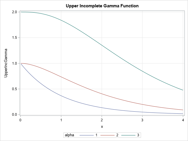
There are two kinds of incomplete gamma functions: the "upper" and the "lower." This article shows how to compute the upper and lower incomplete gamma functions in SAS. A graph of the upper incomplete gamma function is shown to the right for several values of the parameter, α. A graph of the lower incomplete gamma function is shown later in this article.

The gamma function

Before discussing the incomplete gamma function, let's review the "complete" gamma function, which is usually called THE gamma function. The gamma function is defined by the following integral:
$\Gamma(\alpha) = \int_0^{\infty} t^{\alpha-1} e^{-t} \, dt$

Notice that the parameter to the function is α. The integration variable, t, is integrated out and does not appear in the answer. The integral is "complete" because the bounds of integration is the complete positive real line, (0, ∞).

The gamma function generalizes the factorial operation to include positive real numbers. In particular, Γ(1) = 1 and Γ(x+1) = x Γ(x) for any positive real number, x. If n is a positive integer, then Γ(n) = (n-1)!.

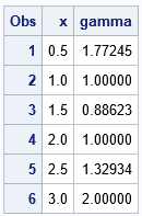
In SAS, you can use the GAMMA function to evaluate the (complete) gamma function at any positive real number:

/* The (complete) gamma function */
data Gamma;
do x = 0.5 to 3 by 0.5;
   gamma = gamma(x);
   output;
end;
run;
 
proc print; run;

The upper and lower incomplete gamma functions

An incomplete gamma function replaces the upper or lower limit of integration in the integral that defines the complete gamma function. If you replace the upper limit of integration (∞) by x, you get the lower incomplete gamma function:
$p(\alpha, x) = \int_0^{x} t^{\alpha-1} e^{-t} \, dt$
Here "lower" refers to integrating only the "left side", which means values of t < x.

If you replace the lower limit of integration (0) by x, you get the upper incomplete gamma function:
$q(\alpha, x) = \int_x^{\infty} t^{\alpha-1} e^{-t} \, dt$
Here "upper" refers to integrating only the "right side", which means values of t > x.

Notice that p(α, x) + q(α, x) = Γ(α) for all values of x. Furthermore, p(α, 0) = 0 and q(α, 0) = Γ(α).

Compute the incomplete gamma function in SAS

The lower incomplete gamma function looks a LOT like the definition of the cumulative distribution function (CDF) of the gamma distribution. The only difference is that the maximum value of a CDF is unity whereas the maximum value of the lower incomplete gamma function is Γ(α). Thus, Γ(α) is a constant scale factor that relates the lower incomplete gamma function and the CDF of the gamma distribution.

Specifically, the CDF function for the gamma distribution with shape parameter α and scale parameter 1 is
$\mbox{CDF}('\mbox{Gamma}', x, \alpha) = \frac{1}{\Gamma(\alpha)} \int_0^x t^{\alpha-1} e^{-t} \, dt$
Equivalently,
$p(\alpha, x) = \Gamma(\alpha) * \mbox{CDF}('\mbox{Gamma}', x, \alpha)$

In the same way, recall that the complementary CDF (sometimes called the survival function or the reliability function) is the quantity SDF(x) = 1 - CDF(x). The SDF of the gamma distribution is a scaled version of the upper incomplete gamma function, as follows:
$q(\alpha, x) = \Gamma(\alpha) * \mbox{SDF}('\mbox{Gamma}', x, \alpha)$

Consequently, you can compute the lower or upper incomplete gamma function in SAS by using the following macros. The SAS DATA step shows how to evaluate the functions on the domain (0, 4] for three values of the parameter, α = 1, 2, and 3. The graphs of the upper incomplete gamma function are shown:

%macro LowerIncGamma(x, alpha); /* lower incomplete gamma function */
   (Gamma(&alpha) * CDF('Gamma', &x, &alpha))
%mend;
%macro UpperIncGamma(x, alpha); /* upper incomplete gamma function */
   (Gamma(&alpha) * SDF('Gamma', &x, &alpha))
%mend;
data IncGamma;
do alpha = 1 to 3;
   do x = 0.01 to 4 by 0.01;
      LowerIncGamma = %LowerIncGamma(x, alpha);
      UpperIncGamma = %UpperIncGamma(x, alpha);
      output;
   end;
end;
run;
 
title "Lower Incomplete Gamma Function";
proc sgplot data=IncGamma;
   series x=x y=LowerIncGamma / group=alpha;
   xaxis grid; yaxis grid;
run;
title "Upper Incomplete Gamma Function";
proc sgplot data=IncGamma;
   series x=x y=UpperIncGamma / group=alpha;
   xaxis grid; yaxis grid;
run;

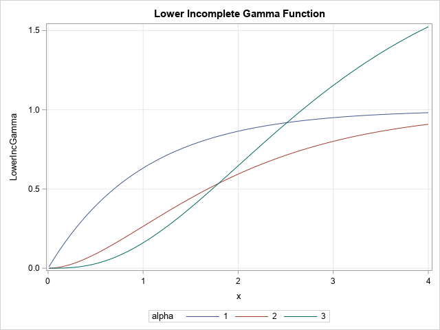
The graph of the upper incomplete gamma function is shown at the top of this article. The following graph shows the lower incomplete gamma function for several values of the α parameter.

By the way, some fields of study will use the term "regularized" incomplete gamma function. The regularized lower incomplete gamma function is simply the CDF of the gamma distribution. The regularized upper incomplete gamma function is the SDF of the gamma distribution.

Summary

As is sometimes the case, different areas of application use different names for essentially the same quantity. Although the SAS language does not provide a built-in function that evaluates the incomplete gamma function, it is easy to evaluate by using the GAMMA and CDF functions, as follows:

The complete gamma function, Γ(α), is computed by using the GAMMA function.
The lower/upper incomplete gamma function is a scaled version of the CDF and SDF (respectively) of the gamma distribution:
- The lower incomplete gamma function is p(alpha,x) = GAMMA(alpha)*CDF('Gamma',x,alpha);
- The upper incomplete gamma function is q(alpha,x) = GAMMA(alpha)*SDF('Gamma',x,alpha);
The lower/upper regularized incomplete gamma function is another named for the CDF and SDF, respectively.
- The regularized lower incomplete gamma function is computed as CDF('Gamma',x,alpha);
- The regularized upper incomplete gamma function is computed as SDF('Gamma',x,alpha);

Blogs