In a previous article, I showed how to perform collinearity diagnostics in SAS by using the COLLIN option in the MODEL statement in PROC REG. For models that contain an intercept term, I noted that there has been considerable debate about whether the data vectors should be mean-centered prior to performing the collinearity diagnostics. In other words, if X is the design matrix used for the regression, should you use X to analyze collinearity or should you use the centered data X – mean(X)? The REG procedure provides options for either choice. The COLLIN option uses the X matrix to assess collinearity; the COLLINOINT option uses the centered data.

As Belsley (1984, p. 76) states, "centering will typically seem to improve the conditioning." However, he argues that running collinearity diagnostics on centered data "gives us information about the wrong problem." He goes on to say, "mean-centering typically removes from the data the interpretability that makes conditioning diagnostics meaningful."

This article looks at how centering the data affects the collinearity diagnostics. Throughout this article, when I say "collinearity diagnostics, I am referring to the variance-decomposition algorithm that is implemented by the COLLIN in PROC REG, which was described in the previous article. Nothing in this article applies to the VIF or TOL options in PROC REG, which provide alternative diagnostics.

The article has two main sections:

• The mathematics behind the COLLIN (and COLLINOINT) options in PROC REG.
• An example of an ill-conditioned linear system that becomes perfectly conditioned if you center the data.

The arguments in this article are taken from the references at the end of this article. This article assumes that you have already read my previous article about collinearity diagnostics.

The mathematics of the COLLIN option

The COLLIN option implements the regression-coefficient variance decomposition due to Belsley and presented in Belsley, Kuh, and Welsch (1980), henceforth, BKW. The collinearity diagnostics algorithm (also known as an analysis of structure) performs the following steps:

1. Let X be the data matrix. If the model includes an intercept, X has a column of ones. BKW recommend that you NOT center X, but if you choose to center X, do it at this step. As a reminder, the COLLIN option in PROC REG does not center the data whereas the COLLINOINT option centers the data.
2. Scale X so that each column has unit length (unit variance).
3. Compute the singular value decomposition of X = UDV`.
4. From the diagonal matrix, D, compute the eigenvalues and condition indices of X`X.
5. Compute P, the matrix of variance-decomposition proportions as described in BKW, p. 105-107.
6. From this information, you can determine whether the regression model suffers from harmful collinearity.

To make sure that I completely understand an algorithm, I like to implement it in the SAS/IML matrix language. The following SAS/IML statements implement the analysis-of-structure method. You can run the program on the same Fitness data that were used in the previous article. The results are the same as from PROC REG.

proc iml;
start CollinStruct(lambda, cond, P,         /* output variables */
                   XVar, opt);              /* input variables  */
 
   /* 1. optionally center the data */
   if upcase(opt) = "NOINT" then 
      X = XVar - mean(XVar);                /* COLLINOINT: do not add intercept, center */
   else
      X = j(nrow(XVar), 1, 1) || XVar;      /* COLLIN: add intercept, do not center */
 
   /* 2. Scale X to have unit column length (unit variance) */
   Z = X / sqrt(X[##, ]);
   /* 3. Obtain the SVD of X and calculate condition indices and the P matrix */
   call svd(U, D, V, Z);
   /* 4. compute the eigenvalues and condition indices of X`X */
   lambda = D##2;                           /* eigenvalues are square of singular values */
   cond = sqrt(lambda[1] / lambda);         /* condition indices */
 
   /* 5. Compute P = matrix of variance-decomposition proportions */
   phi = V##2 / lambda`;          /* divide squared columns by eigenvalues (proportions of each PC) */
   phi_k = phi[,+];               /* for each component, sum across columns */
   P = T( phi / phi_k );          /* create proportions and transpose the result */
finish;
 
/* Perform Regression-Coefficient Variance Decomposition of BKW */
varNames = {RunTime Age Weight RunPulse MaxPulse RestPulse};
use fitness;
   read all var varNames into XVar;
close;
 
/* perform COLLIN analysis */
call CollinStruct(lambda, cond, P,  XVar, "INT");
print "----- Do Not Center the Data (COLLIN) -----", lambda cond;
 
/* perform COLLINOINT analysis */
call CollinStruct(lambda0, cond0, P0,  XVar, "NOINT");
print "----- Center the Data (COLLINOINT) -----", lambda0 cond0;

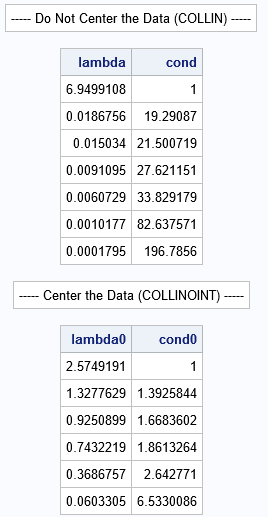
The first table shows the eigenvalues and (more importantly) the condition indices for the original (uncentered) data. You can see that there are three condition indices that exceed 30, which indicates that there might be as many as three sets of nearly collinear relationships among the variables. My previous analysis showed two important sets of relationships:

• Age is moderately collinear with the intercept term.
• RunPulse is strongly collinear with MaxPulse.

In the second table, which analyses the structure of the centered data, none of the condition indices are large. An interpretation of the second table is that the variables are not collinear. This contradicts the first analysis.

Why does centering the data change the condition indices so much? This phenomenon was studied by Belsley who showed that "centering will typically seem to improve the conditioning," sometimes by a large factor (Belsley, 1984, p. 76). Belsley says that the second table "gives us information about the wrong problem; namely, it tells us about the sensitivity of the LS solution... to numerically small relative changes in the centered data. And since the magnitude of the centered changes is usually uninterpretable," so also are the condition indices for the centered data.

Ill-conditioned data that becomes perfectly conditioned by centering

Belsley (1984) presents a small data set (N=20) for which the original variables are highly collinear (maximum condition index is 1,242) whereas the centered data is perfectly conditioned (all condition indices are 1). Belsley could have used a much smaller example, as shown in Chennamaneni et al. (2008). I used their ideas to construct the following example.

Suppose that the (uncentered) data matrix is
X = A + ε B
where A is any N x k matrix that has constant columns, B is a centered orthogonal matrix, and ε > 0 is a small number, such as 0.001. Clearly, X is a small perturbation of a rank-deficient and ill-conditioned matrix (A). The condition indices for X can be made arbitrarily large by making ε arbitrarily small. I think everyone would agree that the columns of X are highly collinear. As shown below, the analysis-of-structure algorithm on X reveals the collinearities.

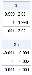
But what happens if you center the data? Because A has constant columns, the mean-centered version of A is the zero matrix. Centering B does not change it because the columns are already centered. Therefore, the centered version of X is ε B, which is a perfectly conditioned orthogonal matrix! This construction is valid for arbitrarily large data, but the following statements implement this construction for a small 3 x 2 matrix.

A = { 1  2,         /* linearly dependent ==> infinite condition index) */
      1  2,
      1  2};
B = {-1  1,         /* orthogonal columns ==> perfect condition number (1) */
      0 -2,
      1  1};
eps = 0.001;        /* the smaller eps is, the more ill-conditioned X is */
X = A + eps * B;    /* small perturbation of a rank deficient matrix */
 
/* The columns of X are highly collinear. The columns X - mean(X) are perfectly conditioned. */
Xc = X - mean(X);
print X, Xc;

This example reveals how "mean-centering can remove from the data the information needed to assess conditioning correctly" (Belsley, 1984, p. 74). As expected, if you run the analysis-of-structure diagnostics on this small example, the collinearity is detected in the original data. However, if you center the data prior to running the diagnostics, the results do not indicate that the data are collinear:

/* The columns of the X matrix are highly collinear, but only 
   the analysis of the uncentered data reveals the collinearity */
call CollinStruct(lambda, cond, P, X, "INT");
print lambda cond P[c={"Intercept" "X1" "X2"}];  /* as ill-conditioned as you want */
 
call CollinStruct(lambda0, cond0, P0, X, "NOINT");
print lambda0 cond0 P0[c={"X1" "X2"}];           /* perfectly conditioned */

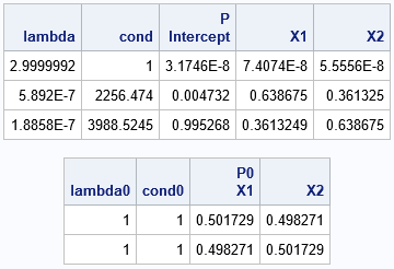
In the first table (which is equivalent to the COLLIN option in PROC REG), the strong collinearities are apparent. In the second table (which is equivalent to the COLLINOINT option), the collinearities are not apparent. As Belsley (1984, p. 75) says, an example like this "demonstrates that it matters very much in what form the data are taken in order to assess meaningfully the conditioning of a LS problem, and that centered data are not usually the correct form."

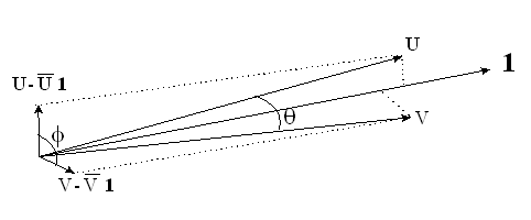
Geometrically, the situation is similar to the following diagram, which is part of Figure 2 on p. 7 of Chennamaneni, et al. (2008). The figure shows two highly collinear vectors (U and V). However, the mean-centered vectors are not close to being collinear and can even be orthogonal (perfectly conditioned).

Summary

In summary, this article has presented Belsley's arguments about why collinearity diagnostics should be performed on the original data. As Belsley (1984, p. 75) says, there are situations in which centering the data is useful, but "assessing conditioning is not one of them." The example in the second section demonstrates why Belsley's arguments are compelling: the data are clearly strongly collinear, yet if you apply the algorithm to the mean-centered data, you do not get any indication that the problem exists. The analysis of the fitness data shows that the same situation can occur in real data.

These examples convince me that the analysis-of-structure algorithm reveals collinearity only when you apply it to the original data. If you agree, then you should use the COLLIN option in PROC REG to perform collinearity diagnostics.

However, not everyone agrees with Belsley. If you are not convinced, you can use the COLLINOINT option in PROC REG to perform collinearity diagnostics on the centered data. However, be aware that the estimates for the centered data are still subject to inflated variances and sensitive parameter estimates (Belsley, 1984, p. 74), even if this diagnostic procedure does not reveal that fact.

Further reading

• Belsley, D. A. (1984). "Demeaning conditioning diagnostics through centering," The American Statistician, 38(2), 73-77. The article is followed by several rejoinders, some of which argue an opposing viewpoint.
• Belsley, D. A., Kuh, E., & Welsch, R. E. (1980). Regression diagnostics: Identifying influential data and sources of collinearity. John Wiley & Sons. A second edition was published in 2004.
• Chennamaneni, P., Echambadi, R., Hess, J. D., and Syam, N. (2008). "How Do You Properly Diagnose Harmful Collinearity in Moderated Regressions?". Retrieved May, 25, 2011.