Influential observations in a linear regression model: The DFBETAS statistics

My article about deletion diagnostics investigated how influential an observation is to a least squares regression model. In other words, if you delete the i_th observation and refit the model, what happens to the statistics for the model? SAS regression procedures provide many tables and graphs that enable you to examine the influence of deleting an observation. For example:

The DFBETAS are statistics that indicate the effect that deleting each observation has on the estimates for the regression coefficients.
The DFFITS and Cook's D statistics indicate the effect that deleting each observation has on the predicted values of the model.
The COVRATIO statistics indicate the effect that deleting each observation has on the variance-covariance matrix of the estimates.

These observation-wise statistics are typically used for smaller data sets (n ≤ 1000) because the influence of any single observation diminishes as the sample size increases. You can get a table of these (and other) deletion diagnostics by using the INFLUENCE option on the MODEL statement of PROC REG in SAS. However, because there is one statistic per observation, these statistics are usually graphed. PROC REG can automatically generate needle plots of these statistics (with heuristic cutoff values) by using the PLOTS= option on the PROC REG statement.

This article describes the DFBETAS statistic and shows how to create graphs of the DFBETAS in PROC REG in SAS. The next article discusses the DFFITS and Cook's D statistics. The COVRATIO statistic is not as popular, so I won't say more about that statistic.

DFBETAS: How the coefficient estimates change if an observation is excluded

The documentation for PROC REG has a section that describes the influence statistics, which is based on the book Regression Diagnostics by Belsley, Kuh, and Welsch (1980, p. 13-14). Among these, the DFBETAS statistics are perhaps the easiest to understand. If you exclude an observation from the data and refit the model, you will get new parameter estimates. How much do the estimates change? Notice that you get one statistic for each observation and also one for each regressor (including the intercept). Thus if you have n observations and k regressors, you get nk statistics.

Typically, these statistics are shown in a panel of k plots, with the DFBETAS for each regressor plotted against the observation number. Because "observation number" is an arbitrary number, I like to sort the data by the response variable. Then I know that the small observation numbers correspond to low values of the response variable and large observation numbers correspond to high values of the response variable. The following DATA step extracts a subset of n = 84 vehicles from the Sashelp.Cars data, creates a short ID variable for labeling observations, and sorts the data by the response variable, MPG_City:

data cars;
set sashelp.cars;
where Type in ('SUV', 'Truck');
/* make short ID label from Make and Model values */
length IDMakeMod $20;
IDMakeMod = cats(substr(Make,1,4), ":", substr(Model,1,5));
run;
 
proc sort data=cars;
   by MPG_City;
run;
 
proc print data=cars(obs=5) noobs;
   var Make Model IDMakeMod MPG_City;
run;

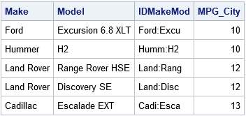
The first few observations are shown. Notice that the first observations correspond to small values of the MPG_City variable. Notice also a short label (IDMakeMod) identifies each vehicle.

There are two ways to generate the DFBETAS statistics: You can use the INFLUENCE option on the MODEL statement to generate a table of statistics, or you can use the PLOTS=DFBETAS option in the PROC REG statement to generate a panel of graphs. The following call to PROC REG generates a panel of graphs. The IMAGEMAP=ON option on the ODS GRAPHICS statement enables you to hover the mouse pointer over an observation and obtain a brief description of the observation:

ods graphics on / imagemap=on;              /* enable data tips (tooltips) */
proc reg data=Cars plots(only) = DFBetas; 
   model MPG_City = EngineSize HorsePower Weight;
   id IDMakeMod;
run; quit;
ods graphics / imagemap=off;

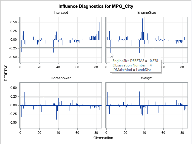
The panel shows the influence of each observation on the estimates of the four regression coefficients. The statistics are standardized so that all graphs can use the same vertical scale. Horizontal lines are drawn at ±2/sqrt(n) ≈ 0.22. Observations are called influential if they have a DFBETA statistic that exceeds that value. The graph shows a tool tip for one of the observations in the EngineSize graph, which shows that the influential point is observation 4, the Land Rover Discovery.

Each graph reveals a few influential observations:

For the intercept estimate, the most influential observations are numbers 1, 35, 83, and 84.
For the EngineSize estimates, the most influential observations are numbers 4, 35, and 38.
For the Horsepower estimates, the most influential observations are numbers 1, 4, and 38.
For the Weight estimates, the most influential observations are numbers 1, 24, 35, and 38.

Notice that several observations (such as 1, 35, and 38) are influential for more than one estimate. Excluding those observations causes several parameter estimates to change substantially.

Labeing the influential observations

For me, the panel of graphs is too small. I found it difficult to hover the mouse pointer exactly over the tip of a needle in an attempt to discover the observation number and name of the vehicle. Fortunately, if you want details like that, PROC REG supplies options that make the process easier. If you don't have too many observations, you can add labels to the DFBETAS plots by using the LABEL suboption. To plot each graph individually (instead of in a panel), use the UNPACK suboption, as follows:

proc reg data=Cars plots(only) = DFBetas(label unpack); 
   model MPG_City = EngineSize HorsePower Weight;
   id IDMakeMod;
quit;

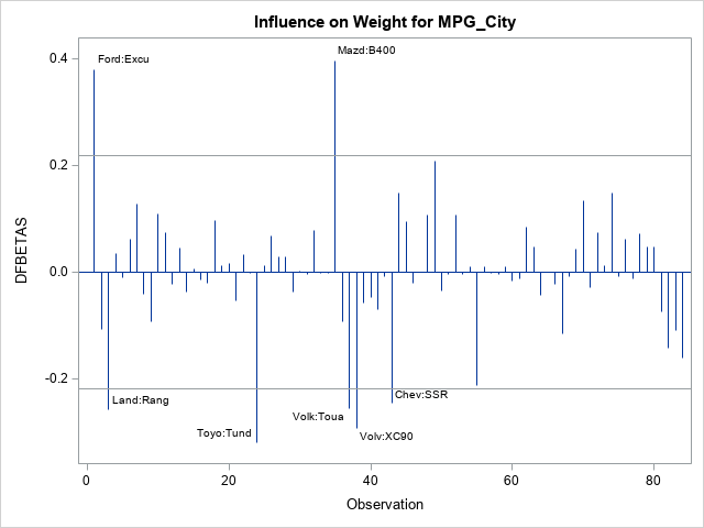
The REG procedure creates four plots, but only the graph for the Weight variable is shown here. In this graph, the influential observations are labeled by the IDMakeMod variable, which enables you to identify vehicles rather than observation numbers. For example, some of the influential observations for the Weight variable are the Ford Excursion (1), the Toyota Tundra (24), the Mazda B400 (35), and the Volvo XC90 (38).

A table of influential observations

If you want a table that displays the most influential observations, you can use the INFLUENCE option to generate the OutputStatistics table, which contains the DFBETAS for all regressors. You can write that table to a SAS data set and exclude any that do not have a large DFBETAS statistic, where "large" means the magnitude of the statistic exceeds 2/sqrt(n), where n is the sample size. The following DATA step filters the observations and prints only the influential ones.

ods exclude all;
proc reg data=Cars plots=NONE; 
   model MPG_City = EngineSize HorsePower Weight / influence;
   id IDMakeMod;
   ods output OutputStatistics=OutputStats;      /* save influence statistics */
run; quit;
ods exclude none;
 
data Influential;
set OutputStats nobs=n;
array DFB[*] DFB_:;
cutoff = 2 / sqrt(n);
ObsNum = _N_;
influential = 0;
DFBInd = '0000';                   /* binary string indicator */
do i = 1 to dim(DFB);
   if abs(DFB[i])>cutoff then do;  /* this obs is influential for i_th regressor */
      substr(DFBInd,i,1) = '1';
      influential = 1;
   end;
end;
if influential;                    /* output only influential obs */
run;
 
proc print data=Influential noobs;
   var ObsNum IDMakeMod DFBInd cutoff DFB_:;
run;

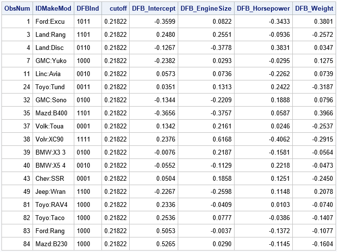
The DFBInd variable is a four-character binary string that indicates which parameter estimates are influenced by each observation. Some observations are influential only for one coefficient; others (1, 3, 35, and 38) are influential for many variables. Creating a binary string for each observation is a useful trick.

By the way, did you notice that the name of the statistic ("DFBETAS") has a large S at the end? Until I researched this article, I assumed it was to make the word plural since there is more than one "DFBETA" statistic. But, no, it turns out that the S stands for "scaled." You can define the DFBETA statistic (without the S) to be the change in parameter estimates b – b(i), but that statistic depends on the scale of the variables. To standardize the statistic, divide by the standard error of the parameter estimates. That scaling is the reason for the S as the end of DFBETAS. The same is true for the DFFITS statistic: S stands for "scaled."

The next article describes how to create similar graphs for the DFFITS and Cook's D statistics.

data have; input x y; datalines; 1 2.89 2 5.87 3 8.98 4 12.20 5 15.06 6 18.03 7 21.15 8 24.08 50 150.00 8 8.00 ; run; proc reg data=have; * N=10; model y = x / influence; run; /* Some results (only those useful for eventually applying the DFBETAS' formula) : beta(x) = 3.01194 DFBETA(x) for the 9th observation = 7.8650 DFBETA(x) for the 10th observation = 4.4307 */ * without the outlier; proc reg data=have; where x NE 50; * N=9; model y = x ; run; /* Some results (only those useful for eventually applying the DFBETAS' formula) : beta(x) = 2.08282 standard error of beta(x) = 0.70514 */ * without the influent observation; proc reg data=have; where y NE 8; * N=9; model y = x ; run; /* Some results (only those useful for eventually applying the DFBETAS' formula) : beta(x) = 3.00003 standard error of beta(x) = 0.00269 */ /* your formula: DFBETA(x) for obs.i = ( beta(X) estimated on all 10 observations - beta(X) estimated on 10 observations except the ith) / standard error of the beta(X) estimated on 10 observations except the ith Calculations: */ %LET beta_X_without_exclusions=3.01194; * from regression-without-exclusions' results; %LET beta_X_outlier_excluded=2.08282; * from regression where the outlier is excluded; %LET std_err_beta_X_outlier_excluded=0.70514; * same provenance; %LET beta_X_influent_excluded=3.00003; * from regression where the influent observation is excluded; %LET std_err_beta_X_influent_excluded=0.00269; * same provenance; DATA _NULL_; DFBETA_X_outlier=%SYSEVALF( (&beta_X_without_exclusions - &beta_X_outlier_excluded) / &std_err_beta_X_outlier_excluded ); PUT DFBETA_X_outlier; DFBETA_X_influent=%SYSEVALF( (&beta_X_without_exclusions - &beta_X_influent_excluded) / &std_err_beta_X_influent_excluded ); PUT DFBETA_X_influent; RUN; /* LOG : 1.3176390504 4.4275092937 */

11 Comments

Pingback: Influential observations in a linear regression model: The DFFITS and Cook's D statistics - The DO Loop
Carlos Alzola on March 26, 2020 10:23 am

Very clear and helpful article. Thank you for publishing it.

Pingback: Identify influential observations in regression models - The DO Loop
Kobina Hagan on April 12, 2021 1:52 am

This is one of the most instructive articles I have ever read. Thank you so much.

Michael O'Neil on September 6, 2021 1:57 am

Rick,

In practical applications with Logistic regressions I have used DFBETAS and have explored a number of alternatives. I have settled on elimination of observations if the observation is influential for more than half of the features in my model. I also push the cut off out beyond the usual xcutoff = 2 / sqrt(n); essentially I am concluding that this cut off is to harsh.

The model is estimated initially to produce the dfbtas, then re-estimated on the training set with the influential observations removed. The impact on the AUR has been significant. The models produced from this approach have been commercially successful where the previous models were not.

There is considerable debate about elimination of data points and many articles I have read would shun my approach.

I would be interested to hear your thoughts on this approach and the debate.

- Rick Wicklin on September 6, 2021 5:55 am
  
  It sounds like you are identifying influential observations. You then eliminate them to obtain a model that has better predictive properties. This ad-hoc process is similar to fitting a robust regression model. Since robust regression has 50+ years of research behind it, I would encourage you to use those techniques. An early SAS paper on robust regression is Chen 2002, which discusses the ROBUSTREG procedure, but there has been a lot of additional progress since then. For generalized linear models, such as logistic regression, some SAS programmers use PROC NLMIXED.
  
  - Michael O'Neil on September 6, 2021 10:10 pm
    
    Thanks Rick, I will investigate further.
    
    - Rick Wicklin on September 7, 2021 10:51 am
      
      I thought more about my response, and I think the question you ask is hard. PROC ROBUSTREG in SAS is restricted to robust linear regression. PROC NLIN or PROC NLMIXED have the potential for Y-robust logistic regression (robust against outliers) but not X-robust logistic regression (robust against influential observations in the explanatory variables), which seems to be the case you are interested in. In the literature, there have been several proposals for robust logistic regression methods. One that has software is
      Cantoni and Ronchetti (2001), “Robust Inference for Generalized Linear Models” and R package: glmrob.
      https://search.r-project.org/CRAN/refmans/robustbase/html/glmrob.html

J.C.Ray on June 22, 2023 6:23 pm

Very clear and helpful article, as usual. Thanks a lot!

I tried to apply the DFBETAS formula you explained in your post "Influential observations in a linear regression model: The DFBETAS statistics",
four years ago (https://blogs.sas.com/content/iml/2019/06/17/influence-regression-dfbeta.html).

I did it on a very simple fictitious dataset, limited to 2 variables (X and Y) and to 10 observations,
where one of which is an outlier without any big effect on the slope of X, and where another one is an influent observation.
I used PROC REG three times: on the whole sample, then on the same sample after having excluded the outlier,
and, finally, on the same sample after having excluded the influent observation.
Combining the relevant pieces of information (the 3 betas for X and their standard errors for the two last models)
within your DFBETAS formula, I got, for the influent observation, the same value (4.43) as the one which is
displayed in the PROC REG's Influence table; but, for the outlier, I got a value (1.317) which is very different from 7.865
(found in the SAS Influence table).
I don't understand why.
Could you tell me why and where I made an error (despite several checks)?
Many thanks

As I apply your formula to the influent observation, I get DFBETA(x)=4.43 (same value as 4.43 in the PROC REG's Influence table).
But, applying it to the outlier, I get DFBETA(x)=1.32, which differs strongly from DFBETA(x)=7.87 displayed by the Influence table.

Rick Wicklin on June 23, 2023 6:20 am

The formula you are using is not correct. The correct formula is shown in the REG doc, which I link to in the first sentence of the second section. When I mentioned at the end of the article that "to standardize the statistic, divide by the standard error of the parameter estimates," I did not intend to imply that the formula is (b - b(i))/StdErr(i), but I see how you could interpret my remark that way. Apologies if my comment about standardization misled you.

J.C.Ray on July 8, 2023 1:18 pm

Thanks to your comment, I was able to calculate the values of DFFITS and DFFBETAS using PROC IML and PROC REG. I'm very grateful.
The calculation of each of the elements used in the formulas for calculating these statistics has enabled me to understand the reasons why an observation which, like the outlier in my data, is not influential in the sense of "modifying the slope of the regression line very much", has a higher DFBETAS than the observation below the rest of the scatter plot, which is clearly influential. I conclude from this that, if the aim is to discard the few observations that have an exaggerated influence on the estimated value of the slope, while keeping the outliers that, located in the extension of the regression line, contribute to the significance of the estimated value of the slope, I must not rely on the highest absolute values of DFBETAS. But maybe I'm wrong. I'd like to hope so.

Blogs