Standardize regression coefficients for models that include categorical variables

A previous article discusses standardized coefficients in linear regression models and shows how to compute standardized regression coefficients in SAS by using the STB option on the MODEL statement in PROC REG. It also discusses how to interpret a standardized regression coefficient.

Recently, a SAS user wanted to know how to get standardized coefficients for regression models that include one or more categorical variables. The user noticed that the GLM procedure in SAS does not support the STB option, and the REG procedure does not directly support categorical variables.

This article discusses the following issues:

How to compute estimates of the standardized regression coefficients by using the STB option on the MODEL statement in PROC GLMSELECT.
How to reproduce the GLMSELECT estimates manually. You can create the design matrix for the regression and use PROC STDIZE to standardize the columns in the design matrix. You can then use PROC REG to reproduce the results of the STB option in PROC GLMSELECT. If you need confidence intervals for the standardized coefficient of a categorical variable, you can use the CLB option in PROC REG.
How to interpret the standardized regression coefficients for categorical variables. Does it make sense to standardize the dummy variables in a design matrix?

You can also read the SAS Usage Note on this topic.

Standardized regression coefficients for continuous variables

Let's quickly review the interpretation of regression coefficients in a linear regression model that has continuous explanatory variables and a continuous response variable. The details are shown in a previous article.

For an unstandardized explanatory variable, you can interpret the regression coefficient as "the expected change in the response for one unit of change in the explanatory variable" while keeping the other variables in the model constant. Notice that this interpretation refers to the scale or units of the explanatory variable. If you change the units of the explanatory variable, the coefficient changes. For example, suppose an explanatory variable represents a length. You can measure the length in centimeters, meters, or even inches. If you choose meters, the regression coefficient will be 100 times larger than if you choose centimeters. If you choose inches, the regression coefficient will be 2.54 times larger than if you choose centimeters.

To make the estimates independent of units, you can standardize the explanatory variable to have unit standard deviation. The resulting parameter estimate is called the standardized regression coefficient. (We often standardize the variable to have zero mean as well.) The interpretation of the standardized regression coefficient is "the expected change in the response for one standard deviation of change in the explanatory variable," while controlling for the other variables.

In SAS, you can obtain the estimates of the standardized regression coefficients by using the STB option on the MODEL statement in PROC REG. Be aware that the STB option also standardizes the response variable. Therefore, the interpretation of a standardized regression coefficient in PROC REG is "the expected number of standard deviations of change in the response for one standard deviation of change in the explanatory variable," while controlling for the other variables.

Because it is cumbersome to always tack on "while controlling for the other variables" to the end of the interpretation, I will drop that phrase for the rest of this article. But you should always mentally include that phrase when you consider the interpretation of a regression coefficient.

Standardized regression coefficients for categorical variables

If your linear regression model contains a categorical variable, you cannot use PROC REG directly. Furthermore, PROC GLM does not support the STB option to display standardized estimates. However, the GLMSELECT procedure does support the STB. Let's run an example. Let's choose one continuous variable and one categorical variable (which has three levels) from the Sashelp.Cars data set. The following call to PROC GLMSELECT displays the standardized regression coefficients. For a future analysis, it uses the OUTDESIGN= option to create an output data set that contains the continuous variables in the model and the dummy variables for the categorical variable, Origin. For more about the OUTDESIGN= option, see "The best way to generate dummy variables in SAS."

/* keep a response variable (MPG_City), a continuous regressor (Horsepower), and a categorical regressor (Origin) */
data Cars;
   set Sashelp.Cars;
   keep MPG_city Horsepower Origin;
run;
 
/* PROC GLMSELECT provides standardized estimates, including for the CLASS variables.
   The coefficients are for the model that standardizes the columns in the design matrix.
   Like the STB option in PROC REG, the response variable is also standardized.
*/
/* Optional: write dummy variables and original variables to the OUTDESIGN= data set for later use */
proc glmselect data=Cars 
               outdesign(addinputvars fullmodel)=GLSDesign;
   class Origin;
   model MPG_city = Horsepower Origin / selection=none STB;     /* standardize Xs and Y */
   ods select ParameterEstimates;
run;

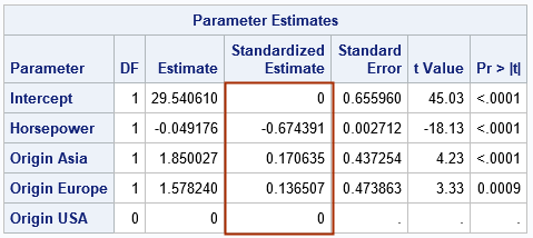
The table shows the parameter estimates and the associated statistics. The column labeled "Standardized Estimate" displays the estimates for the standardized regression coefficients. As explained in the previous article, the standardized Intercept coefficient will always be 0.

By default, the procedure uses the GLM parameterization to create the dummy variables for the CLASS variable, and the last category ('USA') is the reference level. Consequently, the unstandardized estimates indicate the expected change in the response when comparing Origin="Asia' or Origin='Europe' to the reference level. For example, the model predicts that Asia-manufactured cars get an additional 1.85 mile per gallon as compared to their USA-manufactured counterparts.

The standardized estimates for categorical variables are difficult to interpret. I discuss this in a later section. For now, let's just note that response variable is measured in "miles per gallon," which is not a unit that is used in most of the world. You could, of course, convert the response variable to "liters per 100 kilometers" or some other unit, but the standardized coefficients eliminate the units altogether. The magnitude of the standardized estimates tells you something about the relative importance of the effects on the response variable. In some sense, the Horsepower variable is the strongest effect, followed by the Origin='Asia' vehicles, followed by the Origin='Europe' vehicles. The size of the standardized coefficients are used by PROC GLMSELECT during variable selection to display the coefficient progression plot, which shows how the model evolves as effects are added or removed from the model.

Manual calculation of standardized effects

It is useful to understand how PROC GLMSELECT computes the standardized estimates. In short, it uses the columns of the design matrix as if all columns correspond to continuous variables. You can reproduce the standardized estimates by doing the following:

Output the design matrix, including dummy variables for the classification effects. I performed this step in the previous call to PROC GLMSELECT. The design matrix is stored in the GLSDesign data set.
Use PROC STDIZE to standardize the explanatory variables, including the dummy variables. If you want to get the same results as PROC GLMSELECT, you must also standardize the response variable.
Use PROC REG to compute the regression estimates for the standardized columns.

In SAS, you can use the following statements to carry out these steps:

/* Step 1: Use the OUTDESIGN= option in PROC GLMSELECT to output the design matrix. */
 
/* Step 2: Use PROC STDIZE to standardize the explanatory variables, including the dummy variables. */
proc stdize data=GLSDesign out=CarsStd method=std OPREFIX SPREFIX=Std;
   var MPG_city Horsepower Origin_Asia Origin_Europe Origin_USA;
run;
 
/* Step 3: Use PROC REG to compute the parameter estimates for the (standardized) variables. */
options nolabel;   /* suppress labels: blogs.sas.com/content/iml/2012/08/13/suppress-variable-labels-in-sas-procedures.html */
proc reg data=CarsStd plots=none;
   Stdize: model StdMPG_city = StdHorsepower 
                    StdOrigin_Asia StdOrigin_Europe StdOrigin_USA / CLB;    /* use NOINT to get Int=0 */
   ods select ParameterEstimates;
quit;

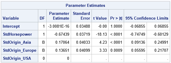
The output shows the standardized coefficients, as well as standard errors and confidence intervals for the standardized coefficients. As far as I know, this "manual" technique is the only way to get confidence intervals for standardized regression coefficients.

Because you know that the Intercept estimate is exactly 0, you can use the NOINT option to exclude the estimate for the Intercept. Similarly, you can exclude the dummy variable for the reference level (in this case, StdOrigin_USA) from the MODEL statement.

Interpretation of standardized coefficients for categorical variables

I'll be frank: If your goal is to obtain an interpretable regression model, I do not advocate standardizing categorical variables. When you standardize a variable, you are using the standard deviation of the data as the unit of scale. But a categorical variable does not have an intrinsic unit of scale. The role of a categorical variable in a regression model is to enable you to compare the effect of different levels of the variable on the response. For example, let C be a categorical variable with levels C1, C2, and C3. If you use the GLM parameterization with reference level C3, the estimate for C1 is the expected change in the response between the subjects with C=C1 as compared to the subjects with C=C3. Similarly, the estimate for C2 is the expected change in the response as compared to the subjects with C=C3. This interpretation is intrinsically linked to the fact that the design matrix contains three binary indicator columns (dummy variables) that correspond to the levels of the categorical variable.

If you standardize dummy variables, you lose this interpretation. Instead, the regression procedure treats the standardized variables as if they were continuous. The standardized regression coefficients is the expected change in the response due to "one standard deviation" of change in the standardized values. However, a categorical variable cannot change by one standard deviation. It can only change from one level to another.

Personally, I think the best way to obtain an interpretable model is to standardize only the continuous variables and to leave the categorical variables unstandardized. To do this, specify the standardized continuous variables and the unstandardized categorical variables on the MODEL statement, as follows:

/* Alternate Step 3: Do not standardize the dummy variables for CLASS variables. */
proc glm data=CarsStd plots=none;
   class Origin;
   model StdMPG_city = StdHorsepower Origin / solution CLPARM;
   ods select ParameterEstimates;
quit;

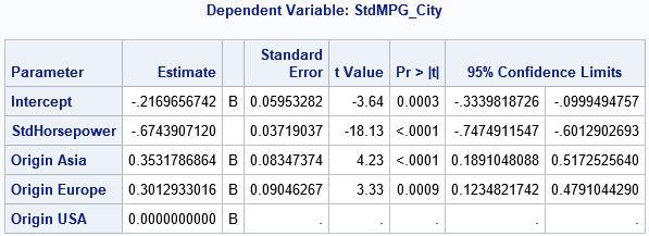
To me, this is the model for which the parameter estimates are most interpretable. For a continuous variable, the coefficient estimate is the "expected number of standard deviations of change in the response for one standard deviation of change in the explanatory variable." For a categorial variable, the coefficient estimate is "expected number of standard deviations of change in the response between subjects at one level as compared to the reference level."

You might ask, "why does SAS compute standardized regression coefficients for the categorical variables if they aren't interpretable?" My answer is that they are useful for variable selection techniques in which you want to keep an effect in a model when the effect improves the prediction of the model. For variable selection techniques, it is useful to have a standardized measure that you can use for all effects, continuous and categorical.

Summary

This article discusses how to use SAS to estimate standardized regression coefficients for linear regression models that include a categorical variable. The easy way to get the estimates is to use PROC GLMSELECT. With a little more work, you can use PROC STDIZE and PROC REG to also get confidence intervals for the standardized coefficients. Lastly, the article discusses the interpretation of the standardized coefficients. When you standardize all variables, you can directly compare the magnitude of each effect. But for categorical variables, a standardized coefficient is not very interpretable, whereas the unstandardized coefficient is. A hybrid model might be the most interpretable: standardize the continuous variables but leave the categorial variables unstandardized.

Blogs