In computational statistics, there are often several ways to solve the same problem. For example, there are many ways to solve for the least-squares solution of a linear regression model. A SAS programmer recently mentioned that some open-source software uses the QR algorithm to solve least-squares regression problems and asked how that compares with SAS. This article shows how to estimate a least-squares regression model by using the QR method in SAS. It shows how to use the QR method in an efficient way.

Solving the least-squares problem

Before discussing the QR method, let's briefly review other ways to construct a least-squares solution to a regression problem. In a regression problem, you have an n x m data matrix, X, and an n x 1 observed vector of responses, y. When n > m, this is an overdetermined system and typically there is no exact solution. Consequently, the goal is to find the m x 1 vector of regression coefficients, b, such that the predicted values (X b) are as close as possible to the observed values. If b is a least-squares solution, then b minimizes the vector norm || X b - y ||², where ||v||² is the sum of the squares of the components of a vector.

Using calculus, you can show that the solution vector, b, satisfies the normal equations (X`X) b = X`y. The normal equations have a unique solution when the crossproduct matrix X`X is nonsingular. Most numerical algorithms for least-squares regression start with the normal equations, which have nice numerical properties that can be exploited.

Creating a design matrix

The first step of solving a regression problem is to create the design matrix. For continuous explanatory variables, this is easy: You merely append a column of ones (the intercept column) to the matrix of the explanatory variables. For more complicated regression models that contain manufactured effects such as classification effects, interaction effects, or spline effects, you need to create a design matrix. The GLMSELECT procedure is the best way to create a design matrix for fixed effects in SAS. The following call to PROC GLMSELECT writes the design matrix to the DesignMat data set. The call to PROC REG estimates the regression coefficients:

proc glmselect data=Sashelp.Class outdesign=DesignMat;  /* write design matrix */
   class Sex;
   model Weight = Height Sex Height*Sex/ selection=none;
run;
/* test: use the design matrix to estimate the regression coefficients */
proc reg data=DesignMat plots=none;
   model Weight = Height Sex_F Height_Sex_F;
run;

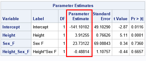
The goal of the rest of this article is to reproduce the regression estimates by using various other linear algebra operations. For each method, we want to produce the same estimates: {-141.10, 3.91, 23.73, -0.49}.

Linear regression: A linear algebraic approach

I've previously discussed the fact that most SAS regression procedures use the sweep operator to construct least-squares solutions. Another alternative is to use the SOLVE function in SAS/IML:

proc iml;
use DesignMat;
   read all var {'Intercept' 'Height' 'Sex_F' 'Height_Sex_F'} into X;
   read all var {'Weight'} into Y;
close;
 
/* form normal equations */
XpX = X`*X;
Xpy = X`*y;
 
/* an efficient numerical solution: solve a particular RHS */
b = solve(XpX, Xpy);
print b[L="SOLVE" F=D10.4];

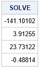
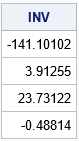
The SOLVE function is very efficient and gives the same parameter estimates as the SWEEP operator (which was used by PROC REG). Using the SOLVE function on the system A*b=z is mathematically equivalent to using the matrix inverse to find b=A^-1z. However, the INV function explicitly forms the inverse matrix, whereas the SOLVE function does not. Consequently, the SOLVE function is faster and more efficient than using the following SAS/IML statement:

/* a less efficient numerical solution */
Ainv = inv(XpX);       /* explicitly form the (m x m) inverse matrix */
b = Ainv*Xpy;          /* apply the inverse matrix to RHS */
print b[L="INV" F=D10.4];

For a performance comparison of the SOLVE and INV functions, see the article, "Solving linear systems: Which technique is fastest?"

An introduction to the QR method for solving linear equations

There are many ways to solve the normal equations. The SOLVE (and INV) functions use the LU decomposition. An alternative is the QR algorithm, which is slower but can be more accurate for ill-conditioned systems. You can apply the QR decomposition to the normal equations or to the original design matrix. This section discusses the QR decomposition of the design matrix. A subsequent article discusses decomposing the data matrix directly.

Let's see how the QR algorithm solves the normal equations. You can decompose the crossproduct matrix as the product of an orthogonal matrix, Q, and an upper-triangular matrix, R. If A = X`X, then A = QR. (I am ignoring column pivoting, which is briefly discussed below.) The beauty of an orthogonal matrix is that the transpose equals the inverse. This means that you can reduce the system A b = (X` y) to a triangular system R b = Q` (X` y), which is easily solved by using the TRISOLV function in SAS/IML.

The SAS/IML version of the QR algorithm is a version known as "QR with column pivoting." Using column pivoting improves solving rank-deficient systems and provides better numerical accuracy. However, when the algorithm uses column pivoting, you are actually solving the system AP = QR, where P is a permutation matrix. This potentially adds some complexity to dealing with the QR algorithm. Fortunately, the TRISOLV function supports column pivoting. If you use the TRISOLV function, you do not need to worry about whether pivoting occurred or not.

Using the QR method in SAS/IML

Recall from the earlier example that it is more efficient to use the SOLVE function than the INV function. The reason is that the INV function explicitly constructs an m x m matrix, which then is multiplied with the right-hand side (RHS) vector to obtain the answer. In contrast, the SOLVE function never forms the inverse matrix. Instead, it directly applies transformations to the RHS vector.

The QR call in SAS/IML works similarly. If you do not supply a RHS vector, v, then the QR call returns the full m x m matrix, Q. You then must multiply Q` v yourself. If you do supply the RHS vector, then the QR call returns Q` v without ever forming Q. This second method is more efficient,

See the documentation of the QR call for the complete syntax. The following call uses the inefficient method in which the Q matrix is explicitly constructed:

/* It is inefficient to factor A=QR and explicitly solve the equation R*b = Q`*c */
call QR(Q, R, piv, lindep, XpX);       /* explicitly form the (m x m) matrix Q */
c = Q`*Xpy;                            /* apply the inverse Q matrix to RHS */
b = trisolv(1, R, c, piv);             /* equivalent to b = inv(R)*Q`*c */
print b[L="General QR" F=D10.4];

In contrast, the next call is more efficient because it never explicitly forms the Q matrix:

/* It is more efficient to solve for a specific RHS */
call QR(c, R, piv, lindep, XpX, ,Xpy); /* returns c = Q`*Xpy */
b = trisolv(1, R, c, piv);             /* equivalent to b = inv(R)*Q`*c */
print b[L="Specific QR" F=D10.4];

The output is not shown, but both calls produce estimates for the regression coefficients that are exactly the same as for the earlier examples. Notice that the TRISOLV function takes the pivot vector (which represents a permutation matrix) as the fourth argument. That means you do not need to worry about whether column pivoting occurred during the QR algorithm.

QR applied to the design matrix

As mentioned earlier, you can also apply the QR algorithm to the design matrix, X, and the QR algorithm will return the least-square solution without ever forming the normal equations. This is shown in a subsequent article, which also compares the speed of the various methods for solving the least-squares problem.

Summary

This article discusses three ways to solve a least-squares regression problem. All start by constructing the normal equations: (X`X) b = X` y. The solution of the normal equations (b) is the vector that minimizes the squared differences between the predicted values, X b, and the observed responses, y. This article discusses

• the SWEEP operator, which is used by many SAS regression procedures
• the SOLVE and INV function, which use the LU factorization
• the QR call, which implements the QR algorithm with column pivoting

A follow-up article compares the performance of these methods and of another QR algorithm, which does not use the normal equations.