The sweep operator performs elementary row operations on a system of linear equations. The sweep operator enables you to build regression models by "sweeping in" or "sweeping out" particular rows of the X`X matrix. As you do so, the estimates for the regression coefficients, the error sum of squares, and the generalized inverse of the system are updated simultaneously. This is true not only for a single response variable but also for multiple responses.

You might remember elementary row operations from when you learned Gaussian elimination, which is a general technique for solving linear systems of equations. Sweeping a matrix is similar to Gaussian elimination, but the sweep operator is most often used to solve least squares problems for the normal equations X`X = X`Y. Therefore, in practice, the sweep operator is usually applied to the rows of a symmetric positive definite system.

How to use the sweep operator to obtain least squares estimates

Before we discuss details of the sweep operator, let's show how it produces regression estimates. The following program uses the SWEEP function in SAS/IML on a six-observation data set from J. Goodnight (1979, p. 153). The first three columns of the matrix M contains the design matrix for the explanatory variables; the first column of M represents the intercept parameter. The last column of the augmented matrix is the response variable. The sweep operator is called on the uncorrected sum of squares and crossproducts matrix (the USSCP matrix), which is computed as M`*M. In block form, the USSCP matrix contains the submatrices X`X, X`Y, Y`X, and Y`Y. The following program sweeps the first three rows of the USSCP matrix:

proc iml;
/*Intercept X1  X2  Y */
M  = {  1   1   1   1,
        1   2   1   3,
        1   3   1   3,
        1   1  -1   2,
        1   2  -1   2,
        1   3  -1   1};
S = sweep(M`*M, 1:3);     /* sweep first three rows (Intercept, X1, X2) */
print S;

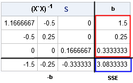
The resulting matrix (S) is divided into blocks by black lines. The leading 3x3 block is the (generalized) inverse of the X`X matrix. The first three elements of the last column (outlined in red) are the least squares estimates for the regression model. The lower right cell (outlined in blue) is the sum of squared errors (SSE) for the regression model.

You can compare the result with the results from PROC REG, as follows. The parameter estimates and error sum of squares are highlighted for easy comparison:

data Have;
input X1 X2 Y @@;
datalines;
1   1   1   2   1   3   3   1   3
1  -1   2   2  -1   2   3  -1   1
;
 
proc reg data=Have USSCP plots=none;
   model Y = X1 X2;
   ods select USSCP ANOVA ParameterEstimates;
run; quit;

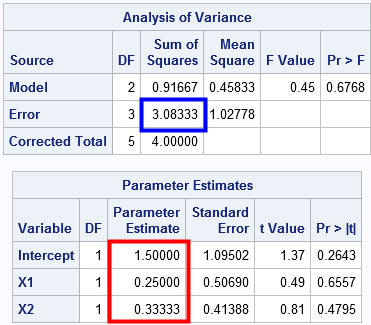
As claimed, the sweep operator produces the same parameter estimates and SSE statistic as PROC REG. The next sections discuss additional details of the sweep operator.

The basics of the sweep operator

Goodnight (1979) defines the sweep operator as the following sequence of row operations. Given a symmetric positive definite matrix A, SWEEP(A, k) modifies the matrix A by using the pivot element A[k,k] and the k_th row, as follows:

1. Let D = A[k,k] be the k_th diagonal element.
2. Divide the k_th row by D.
3. For every other row i ≠ k, let B = A[i,k] be the i_th element of the k_th column. Subtract B x (row k) from row i. Then set A[i,k] = –B/D.
4. Set A[k,k] = 1/D.

You could program these steps in a matrix language such as SAS/IML, but as shown previously, the SAS/IML language supports the SWEEP function as a built-in function.

Sweeping in effects

The following program uses the same data as the first section. The USSCP matrix (S0) represents the normal equations (plus a little extra information). If you sweep the first row of the S0 matrix, you solve the regression problem for an intercept-only model:

proc iml;
/*Intercept X1  X2  Y */
M  = {  1   1   1   1,    1   2   1   3,    1   3   1   3,
        1   1  -1   2,    1   2  -1   2,    1   3  -1   1};
S0 = M`*M;          print S0;   /* USSCP matrix */
 
/* sweep in 1st row (Intercept) */
S1 = sweep(S0, 1);   print S1[F=BEST6.];

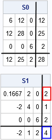
The first element in the fourth row (S1[1,4], outlined in red) is the parameter estimate for the intercept-only model. The last element (S1[4,4], outlined in blue) is the sum of squared errors (SSE) for the intercept-only model.

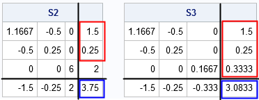
If you "sweep in" the second row, you solve the least squares problem for a model that includes the intercept and X1. The corresponding elements of the last column contain the parameter estimates for the model. The lower-right element again contains the SSE for the revised model. If you proceed to "sweep in" the third row, the last column again contains the parameter estimates and the SSE, this time for the model that includes the intercept, X1, and X2:

/* sweep in 2nd row (X1) and 3rd row (X2) */
S2 = sweep(S1, 2);   print S2[F=BEST6.]; 
S3 = sweep(S2, 3);   print S3[F=BEST6.];

Sweeping out effects

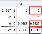
One of the useful features of the sweep operators is that you can remove an effect from a model as easily as you can add it. The sweep operator has a reversibility property: if you sweep a row a second time you "undo" the first sweep. In symbols, the operator has the property that SWEEP( SWEEP(A,k), k) = A for any row k. For example, if you want to take the X1 variable out of the model, merely sweep on the second row again:

S4 = sweep(S3, 2);   print S4[F=BEST6.]; /* model with Intercept + X2 */

Of course, as shown in an earlier section, you do not need to sweep in one row at a time. You can sweep in multiple rows with one call by specifying a vector of indices. In fact, the sweep operator also commutes with itself, which means that you can specify the rows in any order. The call SWEEP(S0, 1:3) is equivalent to SWEEP(S0, {3 1 2}) or SWEEP(S0, {2 3 1}) or any other permutation of {1 2 3}.

Summary

The SWEEP operator (which is implemented in the SWEEP function in SAS/IML) enables you to construct least squares model estimates from the USSCP matrix, which is a block matrix that contains the normal equations. You can "sweep in" rows to add effects to a model or "sweep out" rows to remove effects. After each operation, the parameter estimates appear in the portion of the adjusted USSCP matrix that corresponds to the block for X`Y. Furthermore, the residual sum of squares appears in the portion of the adjusted USSCP matrix that corresponds to Y`Y.

Further reading

The sweep operator is known by different names in different fields and has been rediscovered several times. In statistics, the operator was popularized in a TAS article by J. Goodnight (1979) who mentions Ralston (1960) and Beaton (1964) as early researchers. Outside of statistics, the operator is known as the Principal Pivot Transform (Tucker, 1960), gyration (Duffy, Hazony, and Morrison, 1966), or exchange (Stewart and Stewart, 1998). Tsatsomeros (2000) provides an excellent review of the literature and the history of the sweep operator.

• Goodnight, J. (1979). "A Tutorial on the SWEEP Operator." The American Statistician.
• Tsatsomeros, M. J. (2000). "Principal pivot transforms: properties and applications." Linear Algebra and its Applications.