Compare computational methods for least squares regression

In a previous article, I discussed various ways to solve a least-square linear regression model. I discussed the SWEEP operator (used by many SAS regression routines), the LU-based methods (SOLVE and INV in SAS/IML), and the QR decomposition (CALL QR in SAS/IML). Each method computes the estimates for the regression coefficients, b, by using the normal equations (X`X) b = X`y, where X is a design matrix for the data.

This article describes a QR-based method that does not use the normal equations but works directly with the overdetermined system X b = y. It then compares the performance of the direct QR method to the computational methods that use the normal equations.

The QR solution of an overdetermined system

As shown in the previous article, you can use the QR algorithm to solve the normal equations. However, if you search the internet for "QR algorithm and least squares," you find many articles that show how you can use the QR decomposition to directly solve the overdetermined system X b = y. How does the direct QR method compare to the methods that use the normal equations?

Recall that X is an n x m design matrix, where n > m and X is assumed to be full rank of m. For simplicity, I will ignore column pivoting. If you decompose X = QR_L, the orthogonal matrix Q is n x n, but the matrix R_L is not square. ("L" stands for "long.") However, R_L is the vertical concatenation of a square triangular matrix and a rectangular matrix of zeros:
${\bf R_L} = \begin{bmatrix} {\bf R} \\ {\bf 0} \end{bmatrix}$
If you let Q₁ be the first m columns of Q and let Q₂ be the remaining (n-m) columns, you get a partitioned matrix equation:
$\begin{bmatrix} {\bf Q_1} & {\bf Q_2} \end{bmatrix} \begin{bmatrix} {\bf R} \\ {\bf 0} \end{bmatrix} {\bf b} = {\bf y}$
If you multiply both sides by Q` (the inverse of the orthogonal matrix, Q), you find out that the important matrix equation to solve is ${\bf R b} = {\bf Q_1^{\prime} y}$ . The vector ${\bf Q_1^{\prime} y}$ is the first m rows of the vector ${\bf Q^{\prime} y}$ . The QR call in SAS/IML enables you to obtain the triangular R matrix and the vector Q` y directly from the data matrix and the observed vector. The following program uses the same design matrix as for my previous article. Assuming X has rank m, the call to the QR subroutine returns the m x m triangular matrix, R, and the vector Q` y. You can then extract the first m rows of that vector and solve the triangular system, as follows:

/* Use PROC GLMSELECT to write a design matrix */
proc glmselect data=Sashelp.Class outdesign=DesignMat;
   class Sex;
   model Weight = Height Sex Height*Sex/ selection=none;
run;
 
proc iml;
use DesignMat;
   read all var {'Intercept' 'Height' 'Sex_F' 'Height_Sex_F'} into X;
   read all var {'Weight'} into Y;
close;
 
/* The QR algorithm can work directly with the design matrix and the observed responses. */
call QR(Qty, R, piv, lindep, X, , y);   /* return Q`*y and R (and piv) */
m = ncol(X);
c = QTy[1:m];                           /* we only need the first m rows of Q`*y */
b = trisolv(1, R, c, piv);              /* solve triangular system */
print b[L="Direct QR" F=D10.4];

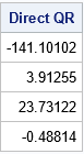
This is the same least-squares solution that was found by using the normal equations in my previous article.

Compare the performance of least-squares solutions

How does this direct method compare with the methods that use the normal equations? You can download a program that creates simulated data and runs each algorithm to estimate the least-squares regression coefficients. The simulated data has 100,000 observations; the number of variables is chosen to be m={10, 25, 50, 75, 100, 250, 500}. The program uses SAS/IML 15.1 on a desktop PC to time the algorithms. The results are shown below:

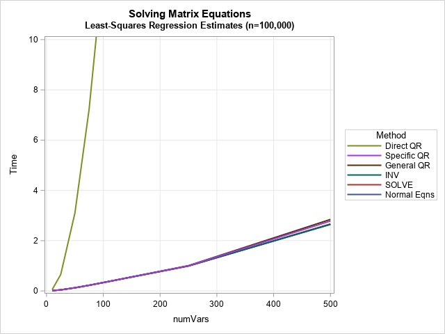
The most obvious feature of the graph is that the "Direct QR" method that is described in this article is not as fast as the methods that use the normal equations. For 100 variables and 100,000 observations, the "Direct QR" call takes more than 12 seconds on my PC. (It's faster on a Linux server). The graph shows that the direct method shown in this article is not competitive with the normal-equation-based algorithms when using the linear algebra routines in SAS/IML 15.1.

The graph shows that the algorithms that use the normal equations are relatively faster. For the SAS/IML calls on my PC, you can compute the regression estimates for 500 variables in about 2.6 seconds. The graph has a separate line for the time required to form the normal equations (which you can think of as forming the X`X matrix). Most of the time is spent computing the normal equations; only a fraction of the time is spent actually solving the normal equations. The following table shows computations on my PC for the case of 500 variables:

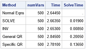
The table shows that it takes about 2.6 seconds to compute the X`X matrix and the vector X`y. After you form the normal equations, solving them is very fast. For this example, the SOLVE and INV methods take only a few milliseconds to solve a 500 x 500. The QR algorithms take 0.1–0.2 seconds longer. So, for this example, forming the normal equations accounts for more than 90% of the total time.

Another article compares the performance of the SOLVE and INV routines in SAS/IML.

SAS regression procedures

These results are not the best that SAS can do. SAS/IML is a general-purpose tool. SAS regression procedures like PROC REG are optimized to compute regression estimates even faster. They also use the SWEEP operator, which is faster than the SOLVE function. For more than 20 years, SAS regression procedures have used multithreaded computations to optimize the performance of regression computations (Cohen, 2002). More recently, SAS Viya added the capability for parallel processing, which can speed up the computations even more. And, of course, they compute much more than only the coefficient estimates! They also compute standard errors, p-values, related statistics (MSE, R square,....), diagnostic plots, and more.

Summary

This article compares several methods for obtaining least-squares regression estimates. It uses simulated data where the number of observations is much greater than the number of variables. It shows that methods that use the normal equations are faster than a "Direct QR" method, which does not use the normal equations. When you use the normal equations, most of the time is spent actually forming the normal equations. After you have done that, the time required to solve the system is relatively fast.

You can download the SAS program that computes the tables and graphs in this article.

Blogs