When fitting a least squares regression model to data, it is often useful to create diagnostic plots of the residuals versus the explanatory variables. If the model fits the data well, the plots of the residuals should not display any patterns. Systematic patterns can indicate that you need to include additional explanatory effects to model the data. Sometimes it is difficult to spot patterns in a seemingly random cloud of points, so some analysts like to add a scatter plot smoother to the residual plots. You can use the SMOOTH suboption to the PLOTS=RESIDUALS option in many SAS regression procedures to generate a panel of residual plots that contain loess smoothers. For SAS procedures that do not support the PLOTS=RESIDUALS option, you can use PROC SGPLOT to manually create a residual plot with a smoother.

Residual plots with loess smoothers

Many SAS linear regression procedures such as PROC REG and PROC GLM support the PLOTS=RESIDUAL(SMOOTH) option on the PROC statement. For example, the following call to PROC GLM automatically creates a panel of scatter plots where the residuals are plotted against each regressor. The model is a two-variable regression of the MPG_City variable in the Sashelp.Cars data.

/* residual plots with loess smoother */
ods graphics on;
proc glm data=Sashelp.Cars plots(only) = Residuals(smooth);
   where Type in ('SUV', 'Truck');
   model MPG_City = EngineSize Weight;
run; quit;

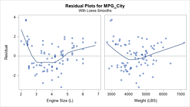
The loess smoothers can sometimes reveal patterns in the residuals that would not otherwise be perceived. In this case, it looks like there is a quadratic pattern to the residuals-versus-EngineSize graph (and perhaps for the Weight variable as well). This indicates that you might need to include a quadratic effect in the model. Because the EngineSize and Weight variables are highly correlated (ρ = 0.81), the following statements add only a quadratic effect for EngineSize:

proc glm data=Sashelp.Cars plots(only) = Residuals(smooth);
   where Type in ('SUV', 'Truck');
   model MPG_City = EngineSize Weight
                    EngineSize*EngineSize ;
quit;

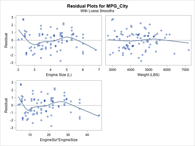
After adding the quadratic effect, the residual plots do not reveal any obvious systematic trends. Also, the residual plot for Weight no longer shows any quadratic pattern.

How to use PROC SGPLOT to create a residual plot with a smoother

If you use a SAS procedure that does not support the PLOTS=RESIDUALS(SMOOTH) option, you can output the residual values to a SAS data set and use PROC SGPLOT to create the residual plots. Even when a procedure DOES support the PLOTS=RESIDUALS(SMOOTH) option, you might want to customize the plot by adding legends, by changing attributes of the markers or curve, or by specifying a value for the smoothing parameter.

An example is shown below. If you use the same model for MPG_City, but use all observations in the data set, the residual plot for EngineSize looks very strange. For these data, the smoothing parameter for the loess curve is very small and therefore the loess curve overfits the residuals:

proc glm data=Sashelp.Cars plots(only) = Residuals(smooth);
   model MPG_City = EngineSize Weight;
   output out=RegOut predicted=Pred residual=Residual;
run; quit;

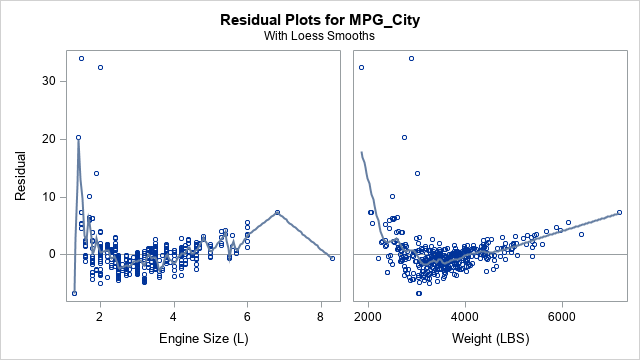
Yuck! The loess curve for the plot on the left clearly overfits the residuals-versus-EngineSize data! Unfortunately, you cannot change the smoothing parameter from the PROC GLM syntax. However, you can change the default smoothing parameter in PROC SGPLOT and you can make other modifications to the plot as well. Notice in the previous call to PROC GLM that the OUTPUT statement creates a data set named RegOut that contains the residual values and the original variables. Therefore, you can create a residual plot and add a loess smoother by using PROC SGPLOT, as follows:

ods graphics / attrpriority=NONE;
title "Residuals for Model";
proc sgplot data=RegOut ;
   scatter x=EngineSize y=Residual / group=Origin;
   loess x=EngineSize y=Residual / nomarkers smooth=0.5;
   refline 0 / axis=y;
   xaxis grid; yaxis grid;
run;

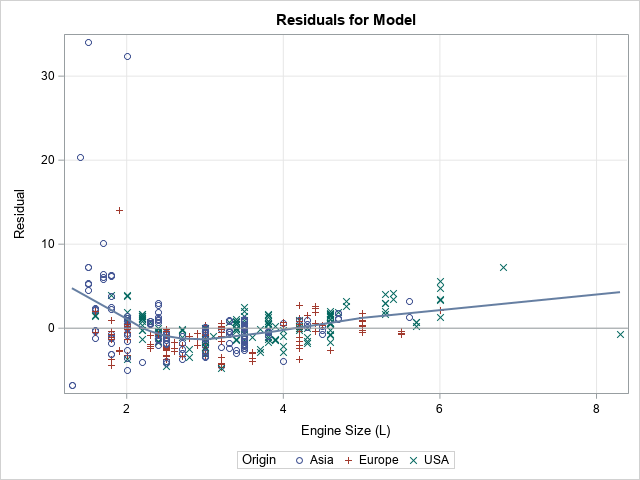
The smoothing parameter was manually set to 0.5, but you can use PROC LOESS if you want to choose a smoothing parameter that optimizes some information criterion such as the AICC statistic. Notice that you can use additional SGPLOT statements to add a reference grid and to change marker attributes. If you prefer, you could add a different kind of smoother such as a penalized B-spline by using the PBSPLINE statement.

You might wonder why the smoother in the residual plot for EngineSize is so small. The parameter is chosen to optimize a criterion such as the AICC statistic, so why does it overfit the data? An example in the PROC LOESS documentation provides an explanation. The chosen value for the smoothing parameter is one that corresponds to a local minimum of an objective function that involves the AICC statistic. Unfortunately, a set of data can have multiple local minima, and this is the case for the residuals of the EngineSize variable. When the smoothing parameter is 0.534, the AICC criterion reaches a local minimum. However, there are smaller values of the smoothing parameter for which the AICC criterion is even smaller. The minimum value of the AICC occurs when the smoothing parameter is 0.015, which leads to the "jagged" loess curve that is seen in the panel of residual plots shown earlier in this section. If you want to see this phenomenon yourself, run the following PROC LOESS code and look at the criterion plot.

ods select CriterionPlot SmoothingCriterion FitPlot;
proc loess data=RegOut;
   model Residual = EngineSize / select=AICC(global) ;
run;

Because a data set can be smoothed at multiple scales, the "optimal" smoothing parameter that is chosen automatically by the PLOTS=RESIDUALS(SMOOTH) option might not enable you to see the general trend of the residuals. If you experience this phenomenon, output the residuals and use PROC SGPLOT or PROC LOESS to compute a more useful smoother.

In summary, SAS provides the PLOTS=RESIDUALS(SMOOTH) option to automatically create residual-versus-regressor plots. Although this panel usually provides a useful indication of patterns in the residuals, you can also output the residuals to a data set and use PROC SGPLOT or PROC LOESS to create a customized residual plot.