An earlier SGMAP blog used the BUBBLE statement to overlay point data on top of an Open Street Map. However, not all map features are points. Some are enclosed areas called polygons. Some map polygons share common borders such as states and counties. Others are separate, non-contiguous regions such as national parks across the country.

The SGMAP procedure requires all polygon data to be in a SAS map data set. The MAPDATA= option in the SGMAP statement specifies that map data set. There are three sources for map data sets. The first two will be covered in future blogs.

1. If you have SAS/GRAPH, worldwide map data from GfK-GeoMarketing® can be part of the SAS installation at your site. If the MAPSGFK library is present, available data sets include continental land masses, country boundaries and internal political subdivisions such as states, counties and provinces. These data sets are updated regularly to reflect name and border changes.
2. You can also download data sets from the original SAS/GRAPH MAPS library from our Maps Online site. They also include similar maps as are in the MAPSGFK library. Although no longer updated they can still provide polygons for a base map.
3. Finally, the MAPIMPORT procedure in Base SAS converts files from Esri™ shapefile format into map data sets. Below we detail the process of importing a shapefile for PROC SGMAP use.

A shapefile is a spatial data format developed by Esri for their GIS software and has become a standard file format for many geospatial packages. When someone speaks of “a shapefile,” they are actually referring to a set of multi-part files having a common file name with various file extensions.

The minimum number of files that comprise a shapefile consists of these file extensions:

.dbf   Attribute data and variable names in dBase format
.shx   Index file
.shp   Feature geometry for points, lines and polygons

Optional shapefile extensions include .xml, .prj, .sbn and .sbx. Shapefiles for specific map features are often zipped together for easier handling and faster downloading.

There is a huge amount of map data on the web with much of it in shapefiles. A few of the many geospatial data portals are:

GeoGratis Canada
Global Map Japan
Czech Republic Geoportal
Philippine GIS Data Clearinghouse
United States Data.gov
Houston, Texas Open Data Portal
Latvia Central Statistics Bureau
New York University Spatial Data Repository
Map Library African Administrative Boundaries
StatSilk Links to Free Shapefile Map Sites
Global Administrative Areas
Free GIS Data Site Collection
U.S. Census Bureau
Statistics Canada

For this example we will use a shapefile of Durham, NC neighborhoods. Durham is one of the cities comprising the Research Triangle. The Durham Neighborhood Compass project displays various lifestyle measurements on an interactive map. That works well for online viewing, but what if you want to generate a map for a static report?

To create your own map you’ll need the polygons defining those neighb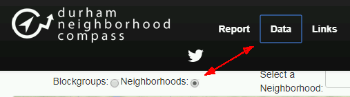orhoods. At the top of the Neighborhood Compass map window select "Neighborhoods" and then click the “Data” button.

From the pop-up menu choose “GIS Shapefile” which is the input format for MAPIMPORT. When the shapefile components download, unzip them to your local disk.

We can now use the MAPIMPORT procedure to convert that shapefile into a SAS map data set. Its syntax has only a few arguments. DATAFILE= is the standard SAS argument which points to the shapefile to import and OUT=  specifies a name for the map data set to create.

proc mapimport
    datafile=’/folders/myfolders/DurhamNeighborhoods_6_12_2015.shp
    out=neighborhoods create_id_;
run;

In order for SGMAP to draw the polygons, it needs to know which variable defines the boundaries. If you are familiar with the variables in the shapefile, or if its metadata specifies one, you can use the ID statement to specify that variable. In this case we are not sure which variable defines the boundaries so we include the CREATE_ID_ option. That adds a variable named _ID_ to the imported map data set with a unique value for each polygon.

Now let's see what the imported map data set WORK.NEIGHBORHOODS looks like.

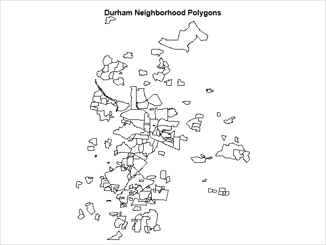
title 'Durham Neighborhood Polygons'; 
proc sgmap mapdata=neighborhoods;
    choromap / mapid=_id_;
run; 

That SGMAP code uses MAPDATA= to specify the map data set. The CHOROMAP statement draws the polygons defined by the _ID_ variable created by MAPIMPORT.

The map at right is exactly what we ordered, a map of the imported polygons with a title, but it's not very useful. It displays the neighborhood polygons but nothing else. As we all know, computers are very literal and do exactly what they are told, which is not always what we really want.

So let's try again and this time add the OPENSTREETMAP statement to plot the polygons on a base map.

title 'Durham Neighborhoods with Open Street Map'; 
proc sgmap mapdata=neighborhoods;
    choromap / mapid=_id_;
    openstreetmap;
run; 

What? This map looks just like the one above. Well, they are not exactly alike. Seeing that the title changed and the log contained no warnings or errors means SGMAP did run..

Oh, it's another example of SGMAP doing exactly what it was told, not what we wanted. Statements are processed in the order submitted. Since the polygons are to be shown on top of the Open Street Map, the CHOROMAP statement must be submitted after OPENSTREETMAP.

This is also the case if you use the ESRIMAP statement. The base map statement must always be first. And this behavior also applies to any BUBBLE, SCATTER or TEXT statements. In order for those map features to be drawn on top of the base map, they must be submitted after it.

So let's try again but submit OPENSTREETMAP before the CHOROMAP statement:

title 'Durham Neighborhoods with Open Street Map';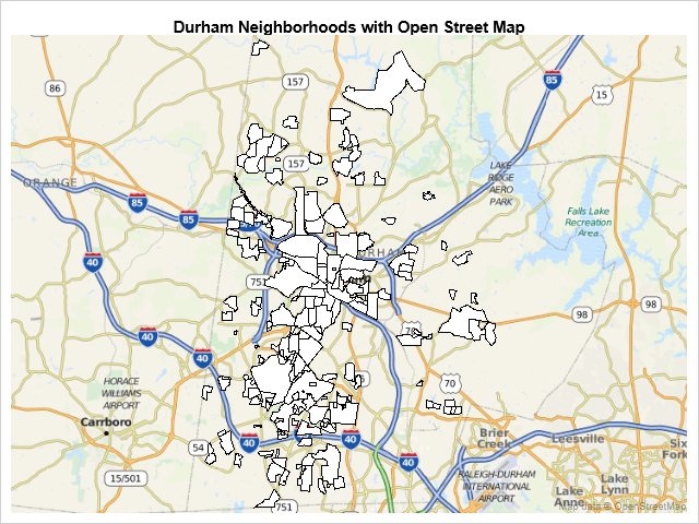 
proc sgmap mapdata=neighborhoods;
    openstreetmap;
    choromap / mapid=_id_;
run; 

Much better. The neighborhoods are now shown on a map of Durham. The Open Street Map tiles were selected automatically using the spatial range of the polygons. We do not want a worldwide map to display features in one city nor do we want polygons hanging off of the base map.

And as a reminder, any coordinates to be plotted on an Open Street Map or Esri map must be unprojected latitude/longitude values. That applies to any CHOROMAP, BUBBLE, SCATTER or TEXT coordinates.

While that last map is better, at least we see the polygons, they do not show us anything except their locations. One of the most helpful things about polygons is their ability to show us something about their respective areas as well as location.

The Compass.SHP.zip file downloaded earlier contained more than shapefiles. It also had a file named CompassDataDictionary_021815.csv. Opening that shows a list of variables with definitions. When the shapefile was imported, those attribute variables were also put into the map data set. So let's look at voting participation in each neighborhood for the 2014 general election which is the PTGNRL_14 variable.

First we need a separate response data set relating voting participation values to the map polygons. Although the PTGNRL_14 values needed are in the imported WORK.NEIGHBORHOODS data set, we do not want to use it for the response data set. It has a lot of observations per polygon which are necessary to draw the polygon borders. While using that data set would work, the data bloat would make the program run really slow.

What we want is a response data set having only one observation per polygon. That's really quite easy with PROC SORT,

proc sort data=neighborhoods out=voting_rates(keep=_id_ ptgnrl_14) nodupkey;
    by _id_;
run; 

The above code reads the WORK.NEIGHBORHOODS map data set, sorts it by the _ID_ variable values, and writes out a new data set named VOTING_RATES. The KEEP option is used to include only the two variables needed: _ID_ and PTGNRL_14.

The key (pun intended) is the NODUPKEY option. It tells PROC SORT to keep only one observation for each unique _ID_ variable value. So NODUPKEY reduces the number of observations from 4528 to 188 or one per polygon. It also decreases the number of variables from 70 to 2. No more data bloat.

Now that we have a proper response data set, let's use it to draw a map with voting rates per neighborhood and also add a legend:

title 'Durham Neighborhood Voting Particpation in 2014';
proc sgmap mapdata=neighborhoods maprespdata=voting_rates;
    openstreetmap;
    choromap ptgnrl_14 / mapid=_id_ name='voting';
    keylegend 'voting';
run;

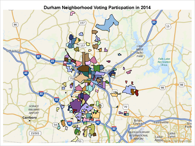
The map certainly looks more interesting, but where is the legend? Our vast SAS coding experience tells us to check the log where we see:

Warning: Legend not shown due to limited available space.

The problem is that the KEYLEGEND statement treats the PTGNRL_14 values as discrete. With 188 discrete observations, no wonder the legend is huge. If it was shown, the map would be the size of a postage stamp, so SGMAP suppresses it and tells you so in the log.

It is just not practical to show most numeric data as discrete unless you have a really limited number of values. Let's set up our own voting percent ranges and categorize each polygon using those ranges. First we create a new response data set using the categories wanted.

data voting_categories (label='General election voting categories');
    set voting_rates;
    length category $16;
    if ptgnrl_14 < 70 then category='<70%';
    else if ptgnrl_14 < 75 then category='70% - 75%';
    else if ptgnrl_14 < 80 then category='75% - 80%';
    else if ptgnrl_14 < 85 then category='80% - 85%';
    else category='>85%';
run;

We next change the code to use that new response data set and its CATEGORY variable.

title 'Durham Neighborhood 2014 General Election';
title2 'Default Style: HTMLBlue';
proc sgmap mapdata=neighborhoods maprespdata=voting_categories;
    openstreetmap;
    choromap category / mapid=_id_ id=_id_ name='voting';
    keylegend 'voting' / title='Participation';
run;

 

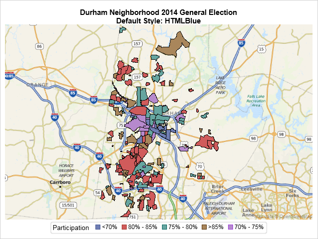
Since we now have a reasonable number of response categories, the map now displays the requested legend.

The default style for the Results output location in SAS Studio is HTMLBlue. When the above code is submitted, SAS Studio uses that style.

 

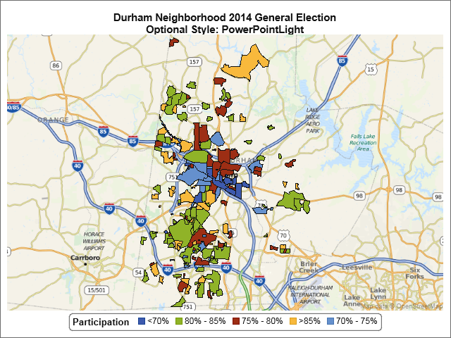
ODS includes a large number of styles. To try a different one, click the SAS Studio options icon and select Preferences. In the Preferences window select the Results option and then use the "HTML output style" pull-down menu to make "PowerPointLight" the new default style. Changing the TITLE2 statement in the previous code and resubmitting it generates the map at right using the PowerPointLight style.

 

Although many styles are available, what if you just prefer to use your own? No problem! Just create a custom style with colors corresponding to the five voting categories. The first color applies to the first category, the second to the second, and so on. You can name the new style anything you wish. For this example we'll call it 'custom_map'.

proc template;
   define Style Styles.custom_map; parent = styles.listing;
       style GraphColors from graphcolors /
            "gdata1"=cxff0000      /* <70% - red */
            "gdata2"=cxffff00        /* 75-75% - yellow */
            "gdata3"=cxffffff         /* 75-80% - white */
            "gdata4"=cx00ffff       /* 80-85% - cyan */
            "gdata5"=cx006600;  /* >85% - dark green */
    end;
run;

Unfortunately it is not possible to use a custom style in the SAS Studio Results output. However we can use it in a different HTML output destination, so we'll open one. Merely wrap the previous SGMAP code with the appropriate ODS statements.

ods html path='/folders/myfolders' (url=none) file='Durham_voting.html' style=custom_map;
ods graphics / imagename='custom_style';
title 'Durham Neighborhood 2014 General Election';
title2 'Style: custom_map';
proc sgmap mapdata=neighborhoods maprespdata=voting_categories;
    openstreetmap;
    choromap category / mapid=_id_ id=_id_ name='voting';
    keylegend 'voting' / title='Participation';
run;
ods html close;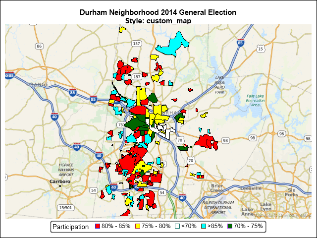

The first ODS HTML statement above specifies the output location and name for the html file. That statement also sets STYLE=CUSTOM_MAP to use the custom style created with PROC TEMPLATE. Then the ODS GRAPHICS statement specifies the name for the output image file containing the map. The final ODS HTML statement closes the output file after SGMAP is done.

When the new code is submitted, the Studio Results output still shows the neighborhood polygons colored by the HTMLBlue style set in Preferences. However, opening the image file in the HTML output path (/folders/myfolders/custom_style.png), we see polygons using the colors in the custom template. Success!

So we now know how to:

1. Import shapefiles to create a SAS map data set,
2. Overlay that data onto an Open Street Map,
3. Display response values in the polygons,
4. Use the standard ODS styles, and
5. Create a custom style for the polygons.

That final program is available here. Details on running it are included in the program comments.

Stay tuned to this channel for more on the SGMAP procedure!