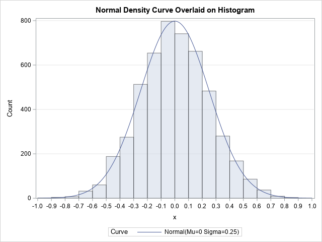
Scale a density curve to match a histogram

This article discusses how to scale a probability density curve so that it fits appropriately on a histogram, as shown in the graph to the right. By definition, a probability density curve is scaled so that the area under the curve equals 1. However, a histogram might show counts or percentages for each bin, so it has a different vertical scale. One way to align these two graphical objects is to rescale the density curve. SAS procedures perform this scaling automatically, but it is helpful to understand how the scaling works. This article explains how to rescale a density curve so that it matches the scale of a histogram. Several examples in SAS help to illustrate the concepts.

Rescale a density estimate

The formula to rescale a density curve is implicitly included in the PROC UNIVARIATE documentation. However, I remember my puzzlement when I first encountered the formulas many years ago. The formulas in the documentation include two symbols that seem out of place: a symbol for the bandwidth (h) of the histogram and a symbol (v) that is related to the VSCALE= option on the HISTOGRAM statement. (If you are unfamiliar with the VSCALE= option, see the appendix.) For example, the following formula specifies the normal density curve that is overlaid on a histogram when you use the NORMAL option on the HISTOGRAM statement:
$p(x) = hv \frac{1}{\sigma \sqrt{2\pi }} \exp \left(-\frac{1}{2} (\frac{x - \mu }{\sigma })^{2}\right)$

Without the h and v symbols, the formula is the normal probability density function with mean μ and standard deviation σ. So why are the symbols h and v present? The answer is that you need these factors to rescale the density function to match the histogram's scale. These symbols also appear in the documentation of other probability distribution and in the formula for a kernel density estimate.

Again, I want to emphasize that SAS performs the scaling automatically. SAS procedures do not require you to perform any manual calculations.

The density scale

A primary use of a histogram is as an empirical estimate for the density of the probability distribution of the data. In physics, we learn that a density is always a ratio. In 3-D, it is mass per unit volume. In 2-D, it is mass per unit area, and in 1-D it is mass per unit length. In statistics, we replace "mass" with "probability." Hence, a one-dimensional probability density for a continuous random variable is probability per unit length.

When histograms are first introduced in school, they are often displayed on the "count scale," which means that the height of each bar represents the number of observations that falls into each histogram bin, which has width h. This scale is used by the histogram at the top of this article. On this scale, the heights of the bars vary between 0 and n, the sample size.

Another popular scale is the proportion scale. Let c[k] be the number of observations in the k_th bin, which is the interval [t, t+h) for some value of t. The proportion c[k]/n estimates the probability that a continuous random variable is in the k_th bin. Therefore, you obtain an estimated probability density by dividing by the length of the bin: (c[k]/n) / h. If f(t) is the underlying probability density function that generates the data, then we expect that (asymptotically) f(t) ≈ c[k]/(nh) when t is inside the k_th bin.

That formula enables us to understand the symbols v and h in the PROC UNIVARIATE documentation:

On the count scale, we want to estimate the count c[k]. The estimate is c[k] ≈ n*h*f(t). Here, v=n.
On the proportion scale, we want to estimate the proportion c[k]/n. Clearly, this equal n*f(t), so set v=1.
A percent is 100% times the proportion. On the percent scale the quantity 100%*c[k]/n is estimated by 100%*n*f(t), so set v=100%.

In all cases, for a histogram that has bin width h, you can align the probability density curve with the histogram by multiplying the curve by v*h and choosing v appropriately.

The role of the bin width in scaling the axis

The appearance of v in the formulas make intuitive sense because you must adjust for the scale of the histogram axis (counts, proportion, or percentage). But what is the intuition behind why the bin width, h, appears as a multiplying factor for the probability density?

To answer that question, let's perform a thought experiment. Suppose you have data that are distributed uniformly on [-1,1]. Suppose you create a histogram on the proportion scale for these data. The heights of the bars depend on the bin size:

If you choose h=0.2, there are 10 bins and each bar is approximately 0.1 units tall.
If you choose h=0.1, there are 20 bins and each bar is approximately 0.05 units tall.
For an arbitrary bin width, h, there are 2/h bins and each bar is approximately h/2 units tall. (This assumes that 2/h is an integer.)

This argument shows that for uniform data, you expect the heights of the bars to be proportional to the bandwidth.

If you prefer to see graphs rather than mathematical arguments, the following SAS statements create a set of uniform data and plot the two histograms. The bin width for the first histogram is twice as big as the second histogram. Accordingly, the bars for the first histogram are approximately twice as tall.

data Unif;
call streaminit(1234);
do i=1 to 5000;
  x = rand("Uniform", -1, 1);
  output;
end;
run;
 
title "Bin Width h=0.2";
proc univariate data=Unif;
  var x;
  histogram x / vscale=proportion endpoints=(-1 to 1 by 0.2) grid odstitle=title;
  ods select histogram;
run;
 
title "Bin Width h=0.1";
proc univariate data=Unif;
  var x;
  histogram x / vscale=proportion endpoints=(-1 to 1 by 0.1) grid odstitle=title;
  ods select histogram;
run;

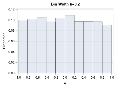
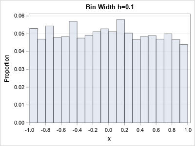
Notice that the first histogram has a vertical axis [0, 0.1] whereas the scale of the second histogram is [0, 0.05].

Areas of bars

Notice that the proportion scale for a histogram is not the same as the natural scale for a probability distribution. For any probability distribution, the area under the curve is exactly 1. However, you can look at the two graphs and see that the area of the bars is not 1.

For h=0.2, there are 10 bars and each bar is approximately 0.1 units tall, so the total area is 10*0.2*0.1 = 0.2.
For h=0.1, there are 20 bars and each bar is approximately 0.05 units tall, so the total area is 20*0.1*0.05 = 0.1.
For an arbitrary bin width, h, there are 2/h bins and each bar is approximately h/2 units tall, so the total area is h. (Again, assuming that 2/h is an integer.)

This explains why h appears as a multiplicative factor when you scale a probability density. I have only presented an intuitive argument for a uniform distribution, but the argument holds more generally. For example, the following SAS code repeats the experiment for normally distributed data:

data Normal;
call streaminit(1234);
do i=1 to 5000;
  x = rand("Normal", 0, 0.25);
  output;
end;
run;
 
title "Bin Width h=0.2";
proc univariate data=Normal;
  var x;
  histogram x / vscale=proportion endpoints=(-1 to 1 by 0.2) grid odstitle=title;
  ods select histogram;
run;
 
title "Bin Width h=0.1";
proc univariate data=Normal;
  var x;
  histogram x / vscale=proportion endpoints=(-1 to 1 by 0.1) grid odstitle=title;
  ods select histogram;
run;

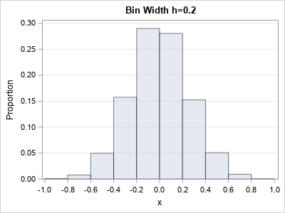
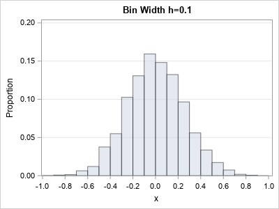
Again, we see that the height of the histogram is proportional the bin width, h. When h is bigger, there are fewer bars, but they tend to be taller. The scale on the first histogram is [0, 0.3]. When h is small, there are more bars, each with a smaller height. The scale on the second histogram is [0, 0.15].

For the proportion scale, the total area of the bars is h. Since the area under a probability density curve is 1, you need to multiply the density curve by h to align it with the histogram on the proportion scale.

Summary

The documentation for PROC UNIVARIATE includes formulas for overlaying a probability density function on a histogram. The formulas all contain scaling parameter h and v, which multiply the density function. This article explains why those parameters are present.

The bandwidth parameter, h: If a histogram displays the proportion of observations in each bin, then the total area of all the bars is h. In comparison, the total area under a density curve is 1. Therefore, you need to multiply the density curve by h if you want to align the curve with a histogram that shows proportions.
The scaling parameter, v: A histogram can display several quantities on the vertical axis: proportion, percentage, or counts. The shape of the histogram does not change, but the vertical axis does. To convert from the proportion scale to the percentage scale, multiply the heights of the bars by 100%. To convert from the proportion scale to the count scale, multiply the heights of the bars by n. The same multiplicative factors apply to scaling a probability density curve.

Appendix: The VSCALE= option

The HISTOGRAM statement in PROC UNIVARIATE supports the VSCALE= option. Valid values for the VSCALE= option are COUNT, PROPORTION, and PERCENT. As the name implies, the VSCALE= option specifies the scale of the vertical scale of the histogram.

When histograms are taught in school, they are often displayed on the "count scale," which means that the height of each bar represents the number of observations that falls into each histogram bin.
If you divide every bar height by n, then the heights represent the proportion of observations that are in each bin. We call this the "proportion scale" for the vertical axis of a histogram. The vertical axis will always be in the range [0,1].
Most people prefer percentages (for example, 20% or 50%) instead of proportions (0.2 or 0.5). If you divide the count in each bin by by n and then multiply by 100%, you obtain the "percent scale." In the percent scale, the heights represent the percentage of observations that are in each bin.

You can control the vertical scale by using the VSCALE= option. By default, VSCALE=PERCENT. Notice that the shape of a histogram does not change when you modify the VSCALE= option. The only thing that changes are the numbers on the vertical axis.

Blogs