A previous article discusses a formula for a confidence interval for R-square in a linear regression model (Olkin and Finn (1995) "Correlations redux", Psychological Bulletin) The formula is useful for large data sets, but should be used with caution for small samples. At the end of the previous article, I stated that an alternative approach is to use bootstrap methods to estimate a confidence interval for R-square. This article shows how to use SAS to bootstrap a confidence interval (CI) for the R-square statistic. It compares the bootstrap CI with the Olkin-Finn CI for a large and a somewhat small sample.

Bootstrap estimate of a regression fit statistic

There are many ways to bootstrap in SAS. For regression models, the most common approach is to use case resampling. However, for many statistics that are associated with a linear regression model, there is a convenient shortcut for generating the bootstrap distributions in SAS: Use the MODELAVERAGE statement in PROC GLMSELECT to perform bootstrap resampling.

To illustrate the bootstrap method, the following SAS statements create a sample of size 10,000 observations from the Sashelp.BWeight data set, which contains data about pregnant mothers and their babies. The call to PROC GLMSELECT fits a regression model for predicting the weight of the baby from an intercept and eight effects: seven main effects and one quadratic interaction.

%let N = 10000;            /* sample size */
data BWeight;
set sashelp.bweight(obs=&N);
keep Weight Black Married Boy MomSmoke CigsPerDay MomAge MomWtGain;
run;
 
proc glmselect data=BWeight seed=12345;
   model Weight = Black Married Boy MomSmoke CigsPerDay 
                  MomAge MomAge*MomAge MomWtGain / selection=none;
   ods select ModelInfo NObs Dimensions FitStatistics;
   ods output FitStatistics=Fit1;
run;

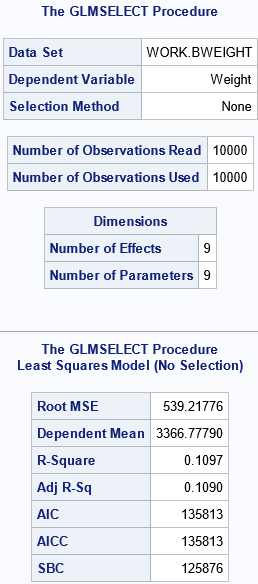
The output shows some information about the data set and the model. There are nine parameters in the model: eight for the specified effects and one for the Intercept for the model. The FitStatistics table shows seven common statistics for linear regression models, including the R-square statistic, which is R² = 0.1097 for this model. The goal of this article is to provide a 95% confidence interval for R².

The bootstrap method can estimate CIs for any of those seven statistics (and for the regression coefficients) so let's put the name of the statistic in a macro variable and put the point estimate into another macro variable. Subsequent statements will refer only to these macro variable, which means that the code in this article can also bootstrap the other fit statistics such as RMSE, Adjusted R-square, AIC, and so forth.

/* put label and value into macro variables */
%let STAT = R-Square; 
data _null_;
   set Fit1;
   where Label1="&STAT";
   call symputx("StatVal", nValue1);
run;
%put &STAT = &StatVal;

   R-Square = 0.1097377994

Bootstrap automatically in PROC GLMSELECT

As mentioned earlier, you can use the MODELAVERAGE statement in PROC GLMSELECT to obtain a bootstrap distribution of the R-square statistic. I am only going to use a small number (B=1,000) of bootstrap resamples because I want to quickly visualize the bootstrap distribution. Because the sample is large (N=10,000) and because the R-square value is not very extreme (R2=0.11), I suspect that the distribution will look approximately normal and be centered near the observed value of R². If so, I can use the Olkin-Finn formula to obtain an asymptotic estimate for the CI. If the distribution does NOT appear to be normal, I won't use the Olkin-Finn formula but instead compute additional bootstrap estimates and obtain a bootstrap CI that has more digits of accuracy.

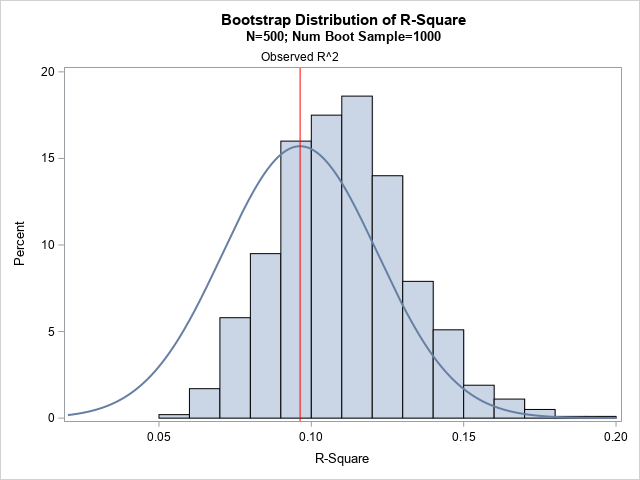
/* Use PROC GLMSELECT for bootstrap estimates and CI of R-square */
%let NumSamples = 1000;       /* number of bootstrap resamples */ 
proc glmselect data=BWeight seed=12345;
   model Weight = Black Married Boy MomSmoke CigsPerDay 
                  MomAge MomAge*MomAge MomWtGain / selection=none;
   modelaverage alpha=0.05 sampling=URS nsamples=&NumSamples /* use URS for bootstrap */
                details tables(only)=(ParmEst); 
   ods select ModelAverageInfo AvgParmEst;        /* display only bootstrap summary */
   ods output FitStatistics=FitStats; /* (SLOW in 9.4!) save bootstrap distribution */
run;
 
/* from the many bootstrap statistics, keep only the R-square statistics */
data MyBootDist;
set FitStats(where=(Label1="&STAT"));
label nValue1="&STAT";
run;
 
title "Bootstrap Distribution of R-Square";
title2 "N=&N; Num Boot Sample=&NumSamples";
proc sgplot data=MyBootDist noautolegend;
   histogram nValue1;
   density nValue1 / type=normal(mu=&StatVal);
   refline &StatVal / axis=x label="Observed R^2" lineattrs=(color=red);
run;

On the MODELAVERAGE statement, I use sampling=URS to obtain bootstrap samples (samples with replacement). I use the DETAILS statement to produce an R-square statistic for each bootstrap sample. The ODS OUTPUT statement writes the 1,000 FitStatistics tables to a data set named FitStats that has 7*1000 observations. I am only interested in the R-square statistic, so I use a DATA step to subset the data. I then call PROC SGPLOT to display a histogram and overlay a normal density curve that is centered at the observed value of R². The graph indicates that the distribution of the R-square statistic appears to be normal, although there seems to be a small bias between the observed statistic and the bootstrap estimate.

Let's use the percentile method to estimate a 95% bootstrap confidence interval. The lower limit of the CI is estimated by the 2.5th percentile of the bootstrap estimates. The upper limit is estimated by the 97.5th percentile. You can use PROC UNIVARIATE to estimate these quantiles:

/* Use approx sampling distribution to make statistical inferences */
proc univariate data=MyBootDist noprint;
   var nValue1;
   output out=Pctl mean=BootR2 std=BootSE 
          /* compute 95% bootstrap confidence interval */
          pctlpre =Boot_  pctlpts =2.5 97.5  pctlname=LCL UCL;
run;
 
proc print data=Pctl noobs; run;

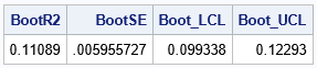
According to this small bootstrap computation, an estimate for the standard error of R-square is 0.006. An estimate for a 95% confidence interval is [0.01, 0.123].

Because the distribution seems to be approximately normal, the next section computes the same quantities by using the Olkin-Finn formula.

Applying the Olkin-Finn formula

The Olkin-Finn formula is an asymptotic (large sample) formula that assumes that the R-square statistic is normal and centered at the observed value of R². Both of these assumptions appear to be satisfied here. To apply the Olkin-Finn formula to obtain a 100(1-α)% confidence interval, you need to supply the following information:

• The sample size, n. In this example, n = 10000.
• The number of explanatory effects in the model, not counting the intercept. In this example, k = 8.
• The point estimate of R² from the data. In this example, R² = 0.1097. That value is stored in the StatVal macro variable.

The following DATA step applies the Olkin-Finn formula:

/* apply the Olkin-Finn formula */
data AsympR2;
alpha = 0.05;        /* obtain 100*(1-alpha)% confidence interval */
n = &N;              /* sample size */
k = 8;               /* number of parameters, not including intercept */
R2 = &StatVal;       /* observed R^2 for sample */
 
SE = sqrt((4*R2*((1-R2)**2)*((n-k-1)**2))/((n**2-1)*(n + 3)));
/* use normal quantile to estimate CI (could also use t quantile) */
z = quantile("Normal", 1-alpha/2);
OF_LCL = R2 - z*SE;   
OF_UCL = R2 + z*SE;
run;
 
title "Asymptotic Confidence Interval for R-Square";
proc print noobs data=AsympR2; 
   var R2 SE OF_LCL OF_UCL;
run;

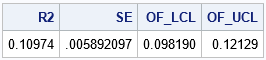
For this regression model, the Olkin-Finn estimate of the standard error of R-square is 0.006. An estimate for a 95% CI is [0.01, 0.121]. This estimate for the standard error is the same as the bootstrap estimate. The lower confidence limit is also the same. The upper confidence limits are almost the same (0.123 versus 0.121). Thus, the Olkin-Finn estimates and the bootstrap estimates are very close to each other for these data and for this model.

Bootstrap estimates for a smaller sample

The Olkin-Finn formula should be used for large samples. What happens if we reduce the size of the sample? To investigate this question, change the sample size by specifying the macro value of N:

%let N = 500;     /* new sample size */

The rest of the program does not need to be modified. When you rerun the program, you get the following histogram that shows the bootstrap distribution versus a normal approximation centered at the observed R² value.

For this sample, there is a large bias between the observed R² value and the mean of the bootstrap distribution. (The distribution also appears to be slightly skewed to the right.) The Olkin-Finn formula incorporates that bias. Whereas the bootstrap estimate of the CI is [0.072, 0.156], the Olkin-Finn estimate is [0.048, 0.144], which is shifted to the left. In this case, I would recommend using a bootstrap estimate of the CI instead of using the Olkin-Finn estimate.

Summary

This article shows how to use the MODELAVERAGE statement in PROC GLMSELECT in SAS to obtain bootstrap estimates for the standard error and confidence interval for the R-square statistic in a linear regression model. With a minor modification, the same program enables you to bootstrap other common fit statistics, such as RMSE or AIC. The bootstrap estimates make very few assumptions and are valid for both large and small samples.

The article also compares the bootstrap estimates to estimates from the Olkin-Finn formula. The Olkin-Finn estimates are intended for large samples and assume that the sampling distribution of the R-square statistic is normal. Furthermore, bias can be an issue when applying the Olkin-Finn formula. I suggest performing a small bootstrap analysis first to check if the bootstrap distribution of the R-square statistic appears to be normal and is centered at the observed value.