A common question is "how do I compute a bootstrap confidence interval in SAS?" As a reminder, the bootstrap method consists of the following steps:

1. Compute the statistic of interest for the original data
2. Resample B times from the data to form B bootstrap samples. How you resample depends on the null hypothesis that you are testing.
3. Compute the statistic on each bootstrap sample. This creates the bootstrap distribution, which approximates the sampling distribution of the statistic under the null hypothesis.
4. Use the approximate sampling distribution to obtain bootstrap estimates such as standard errors, confidence intervals, and evidence for or against the null hypothesis.

The papers by Cassell ("Don't be Loopy", 2007; "BootstrapMania!", 2010) describe ways to bootstrap efficiently in SAS. The basic idea is to use the DATA step, PROC SURVEYSELECT, or the SAS/IML SAMPLE function to generate the bootstrap samples in a single data set. Then use a BY statement to carry out the analysis on each sample. Using the BY-group approach is much faster than using macro loops.

To illustrate bootstrapping in Base SAS, this article shows how to compute a simple bootstrap confidence interval for the skewness statistic by using the bootstrap percentile method. The example is adapted from Chapter 15 of Simulating Data with SAS, which discusses resampling and bootstrap methods in SAS. SAS also provides the %BOOT and %BOOTCI macros, which provide bootstrap methods and several kinds of confidence intervals.

The accuracy of a statistical point estimate

The following statements define a data set called Sample. The data are measurements of the sepal width for 50 randomly chosen iris flowers of the species iris Virginica. The call to PROC MEANS computes the skewness of the sample:

data sample(keep=x);
   set Sashelp.Iris(where=(Species="Virginica") rename=(SepalWidth=x));
run;
 
/* 1. compute value of the statistic on original data: Skewness = 0.366 */
proc means data=sample nolabels Skew;  var x;  run;

The sample skewness for these data is 0.366. This estimates the skewness of sepal widths in the population of all i. Virginica. You can ask two questions: (1) How accurate is the estimate, and (2) Does the data indicate that the distribution of the population is skewed? An answer to (1) is provided by the standard error of the skewness statistic. One way to answer question (2) is to compute a confidence interval for the skewness and see whether it contains 0.

PROC MEANS does not provide a standard error or a confidence interval for the skewness, but the next section shows how to use bootstrap methods to estimate these quantities.

Resampling with PROC SURVEYSELECT

For many resampling schemes, PROC SURVEYSELECT is the simplest way to generate bootstrap samples. The following statements generate 5000 bootstrap samples by repeatedly drawing 50 random observations (with replacement) from the original data:

%let NumSamples = 5000;       /* number of bootstrap resamples */
/* 2. Generate many bootstrap samples */
proc surveyselect data=sample NOPRINT seed=1
     out=BootSSFreq(rename=(Replicate=SampleID))
     method=urs              /* resample with replacement */
     samprate=1              /* each bootstrap sample has N observations */
     /* OUTHITS                 option to suppress the frequency var */
     reps=&NumSamples;       /* generate NumSamples bootstrap resamples */
run;

The output data set represents 5000 samples of size 50, but the output data set contains fewer than 250,000 observations. That is because the SURVEYSELECT procedure generates a variable named NumberHits that records the frequency of each observation in each sample. You can use this variable on the FREQ statement of many SAS procedures, including PROC MEANS. If the SAS procedure that you are using does not support a frequency variable, you can use the OUTHITS option on the PROC SURVEYSELECT statement to obtain a data set that contains 250,000 observations.

BY group analysis of bootstrap samples

The following call to PROC MEANS computes 5000 skewness statistics, one for each of the bootstrap samples. The NOPRINT option is used to suppress the results from appearing on your monitor. (You can read about why it is important to suppress ODS during a bootstrap computation.) The 5000 skewness statistics are written to a data set called OutStats for subsequent analysis:

/* 3. Compute the statistic for each bootstrap sample */
proc means data=BootSSFreq noprint;
   by SampleID;
   freq NumberHits;
   var x;
   output out=OutStats skew=Skewness;  /* approx sampling distribution */
run;

Visualize the bootstrap distribution

The bootstrap distribution tells you how the statistic (in this case, the skewness) might vary due to random sampling variation. You can use a histogram to visualize the bootstrap distribution of the skewness statistic:

title "Bootstrap Distribution";
%let Est = 0.366;
proc sgplot data=OutStats;
   label Skewness= ;
   histogram Skewness;
   /* Optional: draw reference line at observed value and draw 95% CI */
   refline &Est / axis=x lineattrs=(color=red) 
                  name="Est" legendlabel="Observed Statistic = &Est";
   refline -0.44737 0.96934  / axis=x lineattrs=(color=blue) 
                  name="CI" legendlabel="95% CI";
   keylegend "Est" "CI";
run;

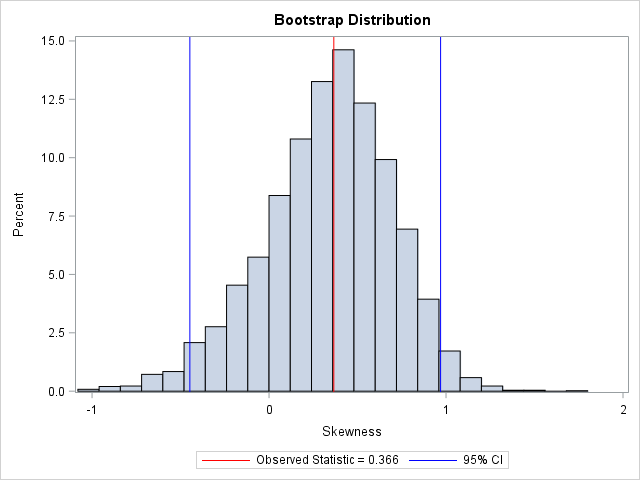
In this graph, the REFLINE statement is used to display (in red) the observed value of the statistic for the original data. A second REFLINE statement plots (in blue) an approximate 95% confidence interval for the skewness parameter, which is computed in the next section. The bootstrap confidence interval contains 0, thus you cannot conclude that the skewness parameter is significantly different from 0.

Compute a bootstrap confidence interval in SAS

The standard deviation of the bootstrap distribution is an estimate for the standard error of the statistic. If the sampling distribution is approximately normal, you can use this fact to construct the usual Wald confidence interval about the observed value of the statistic. That is, if T is the observed statistic, then the endpoints of the 95% two-sided confidence interval are T ± 1.96 SE. (Or use the so-called bootstrap t interval by replacing 1.96 with t_{α/2, n-1}.) The following call to PROC MEANS produces the standard error (not shown):

proc means data=OutStats nolabels N StdDev;
   var Skewness;
run;

However, since the bootstrap distribution is an approximate sampling distribution, you don't need to rely on a normality assumption. Instead, you can use percentiles of the bootstrap distribution to estimate a confidence interval. For example, the following call to PROC UNIVARIATE computes a two-side 95% confidence interval by using the lower 2.5th percentile and the upper 97.5th percentile of the bootstrap distribution:

/* 4. Use approx sampling distribution to make statistical inferences */
proc univariate data=OutStats noprint;
   var Skewness;
   output out=Pctl pctlpre =CI95_
          pctlpts =2.5  97.5       /* compute 95% bootstrap confidence interval */
          pctlname=Lower Upper;
run;
 
proc print data=Pctl noobs; run;

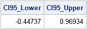
As mentioned previously, the 95% bootstrap confidence interval contains 0. Although the observed skewness value (0.366) might not seem very close to 0, the bootstrap distribution shows that there is substantial variation in the skewness statistic in small samples.

The bootstrap percentile method is a simple way to obtain a confidence interval for many statistics. There are several more sophisticated methods for computing a bootstrap confidence interval, but this simple method provides an easy way to use the bootstrap to assess the accuracy of a point estimate. For an overivew of bootstrap methods, see Davison and Hinkley (1997) Bootstrap Methods and their Application.