If you want to bootstrap the parameters in a statistical regression model, you have two primary choices. The first is case resampling, which is also called resampling observations or resampling pairs. In case resampling, you create the bootstrap sample by randomly selecting observations (with replacement) from the original data. The second choice is called resampling residuals. In this method, you fit a model to the original data to obtain predicted values and residuals. You create the bootstrap sample by using the original explanatory variables but construct a new response value by adding a random residual to the predicted value. This article shows an example of case resampling in SAS. A future article shows an example of resampling residuals.

Case resampling for bootstrapping a regression analysis

If you have some experience with bootstrapping univariate statistics, case resampling will look familiar. The main ideas behind bootstrapping are explained in the article "Compute a bootstrap confidence interval in SAS," which discusses the following steps of the bootstrap method:

1. Compute the statistic of interest for the original data
2. Resample B times from the data to form B bootstrap samples.
3. Compute the statistic on each bootstrap sample. This creates the bootstrap distribution, which approximates the sampling distribution of the statistic.
4. Use the approximate sampling distribution to obtain bootstrap estimates such as standard errors, confidence intervals, and evidence for or against the null hypothesis.

To demonstrate case resampling, consider the sampling distribution of the parameter estimates (the regression coefficients) in an ordinary least squares (OLS) regression. The sampling distribution gives insight into the variation of the estimates and how the estimates are correlated. In a case-resampling analysis, each bootstrap sample will contain randomly chosen observations from the original data. You fit the same regression model to each sample to obtain the bootstrap estimates. You can then analyze the distribution of the bootstrap estimates.

For the statistics in this article, you can compare the bootstrap estimates with estimates of standard errors and confidence intervals (CIs) that are produced by PROC REG in SAS. The procedure constructs the statistics based on several assumptions about the distribution of the errors in the OLS model. In contrast, bootstrap estimates are nonparametric and rely on fewer assumptions. Thus bootstrapping is useful when you are not sure whether the OLS assumptions hold for your data, or when you want to obtain confidence intervals for statistics (like the R-squared and RMSE) that have complicated or unknown sampling distributions.

The statistic of interest for the original data

This example analyzes the Sashelp.Class data set, which contains data about the weights and heights of 19 students. The response variable is the Weight variable, which you can regress onto the Height variable. The regression produces two parameter estimates (Intercept and Height), standard errors, and an estimate of the "covariance of the betas." For clarity, I rename the response variable to Y and the explanatory variable to X so that each variable's role is obvious.

/* regression bootstrap: case resampling */
data sample(keep=x y);
   set Sashelp.Class(rename=(Weight=Y Height=X));  /* rename to make roles easier to understand */
run;
 
/* 1. compute the statistics on the original data */
proc reg data=Sample plots=none;
   model Y = X / CLB covb;                          /* original estimates */
run; quit;

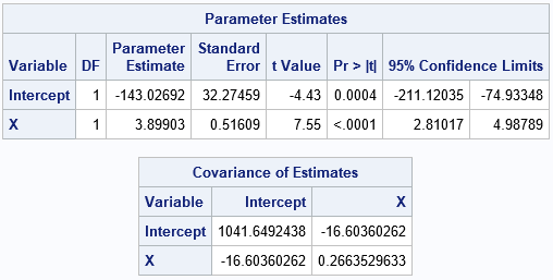
The "Parameter Estimates" table includes point estimates, standard errors, and confidence intervals for the regression coefficients. The "Covariance of Estimates" table shows that the estimates are negatively correlated.

Resample from the data

The following call to PROC SURVEYSELECT creates 5,000 bootstrap samples by sampling with replacement from the data:

title "Bootstrap Distribution of Regression Estimates";
title2 "Case Resampling";
%let NumSamples = 5000;       /* number of bootstrap resamples */
%let IntEst = -143.02692;     /* original estimates for later visualization */
%let XEst   =    3.89903;
 
/* 2. Generate many bootstrap samples by using PROC SURVEYSELECT */
proc surveyselect data=sample NOPRINT seed=1
     out=BootCases(rename=(Replicate=SampleID))
     method=urs              /* resample with replacement */
     samprate=1              /* each bootstrap sample has N observations */
     /* OUTHITS                 use OUTHITS option to suppress the frequency var */
     reps=&NumSamples;       /* generate NumSamples bootstrap resamples */
run;

The output from the SURVEYSELECT procedure is a large data set (BootCases) that contains all bootstrap samples. The SampleID variable indicates which observations belong to each sample. The NumberHits variable gives the frequency for which each of the original observations is selected. That variable should be used as a FREQ variable when analyzing the bootstrap samples. (If your procedure does not have support for a frequency variable, use the OUTHITS option on the PROC SURVEYSELECT statement to obtain an "expanded" version of the bootstrap samples.)

Compute the bootstrap distribution

The BootCases data set contains 5,000 bootstrap samples. You can perform 5,000 regression analyses efficiently by using a BY-group analysis. You can use the BY statement in PROC REG. Be sure to use the NOPRINT option to suppress the output to the screen and use the OUTEST= option to create an output data set that contains 5,000 parameter estimates, one for each bootstrap sample.

/* 3. Compute the statistic for each bootstrap sample */
proc reg data=BootCases outest=PEBoot noprint;
   by SampleID;
   freq NumberHits;
   model Y = X;
run;quit;

Analyze the bootstrap distribution

The PEBoot data set contains 5,000 parameter estimates. To visualize the bootstrap distribution, you can create a scatter plot. The following call to PROC SGPLOT overlays reference lines that intersect at the parameter estimates for the original data.

/* 4. Visualize bootstrap distribution */
proc sgplot data=PEBoot;
   label Intercept = "Estimate of Intercept" X = "Estimate of Coefficient of X";
   scatter x=Intercept y=X / markerattrs=(Symbol=CircleFilled) transparency=0.7;
   /* Optional: draw reference lines at estimates for original data */
   refline &IntEst / axis=x lineattrs=(color=blue);
   refline &XEst / axis=y lineattrs=(color=blue);
   xaxis grid; yaxis grid;
run;

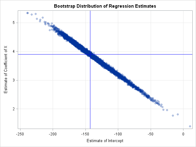
The scatter plot shows that the estimates are negatively correlated, which was previously shown by the output from the COVB option on the original data. You can call PROC CORR on the bootstrap samples to obtain a bootstrap estimate of the covariance of the betas:

proc corr data=PEBoot cov vardef=N;
   var Intercept X;
run;

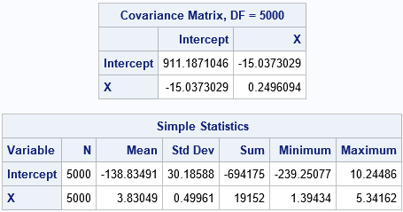
The covariance matrix for the bootstrap estimates is close to the COVB matrix from PROC REG. The "Simple Statistics" table shows other bootstrap estimates. The Mean column shows the average of the bootstrap estimates; the difference between the original parameter estimates and the bootstrap average is an estimate of bias. The StdDev column estimates the standard errors of the regression estimates.

You can also use the 0.025 and 0.975 quantiles of the bootstrap estimates to construct a 95% confidence interval for the parameters. There are many ways to get the percentiles in SAS. the following statements call PROC STDIZE and print the confidence intervals for the Intercept and X variables:

proc stdize data=PEBoot vardef=N pctlpts=2.5 97.5  PctlMtd=ORD_STAT outstat=Pctls;
   var Intercept X;
run;
proc report data=Pctls nowd;
  where _type_ =: 'P';
  label _type_ = 'Confidence Limit';
  columns ('Bootstrap Confidence Intervals (B=5000)' _ALL_);
run;

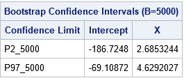
The bootstrap estimates of the confidence intervals are shorter than the Wald confidence intervals from PROC REG that assume normality of errors.

Summary

In summary, there are two primary ways to perform bootstrapping for parameters in a regression model. This article generates bootstrap samples by using "case resampling" in which observations are randomly selected (with replacement). The bootstrap process enables you to estimate the standard errors, confidence intervals, and covariance (or correlation) of the estimates. You can also use the %BOOT macro to carry out this kind of bootstrap analysis.

Case resampling is a good choice when you are modeling observational data in which the explanatory variables are observed randomly from a population. Although OLS regression treats the explanatory variable (such as Height) as a fixed effect, if you were to go into a different school and randomly select 19 students from the same grade, you would obtain a different set of heights. In that sense, the data (X and Y) can be thought of as random values from a larger population.

If you are analyzing data from a designed experiment in which the explanatory variables have a small number of specified values, you can use residual resampling, which is discussed in the next blog post.