Since the late 1990s, SAS has supplied macros for basic bootstrap and jackknife analyses. This article provides an example that shows how to use the %BOOT and %BOOTCI macros. The %BOOT macro generates a bootstrap distribution and computes basic statistics about the bootstrap distribution, including estimates of bias, standard error, and a confidence interval that is suitable when the sampling distribution is normally distributed. Because bootstrap methods are often used when you do not want to assume a statistic is normally distributed, the %BOOTCI macro supports several additional confidence intervals, such as percentile-based and bias-adjusted intervals.

You can download the macros for free from the SAS Support website. The website includes additional examples, documentation, and a discussion of the capabilities of the macros.

The %BOOT macro uses simple uniform random sampling (with replacement) or balanced bootstrap sampling to generate the bootstrap samples. It then calls a user-supplied %ANALYZE macro to compute the bootstrap distribution of your statistic.

How to install and use the %BOOT and %BOOTCI macros

To use the macros, do the following:

1. Download the source file for the macros and save it in a directory that is accessible to SAS. For this example, I saved the source file to C:\Temp\jackboot.sas.
2. Define a macro named %ANALYZE that computes the bootstrap statistic from a bootstrap sample. The next section provides an example.
3. Call the %BOOT macro. The %BOOT macro creates three primary data sets:
   • BootData is a data set view that contains B bootstrap samples of the data. For this example, I use B=5000.
   • BootDist is a data set that contains the bootstrap distribution. It is created when the %BOOT macro internally calls the %ANALYZE macro on the BootData data set.
   • BootStat is a data set that contains statistics about the bootstrap distribution. For example, the BootStat data set contains the mean and standard deviation of the bootstrap distribution, among other statistics.
4. If you want confidence inervals, use the %BOOTCI macro to compute up to six different interval estimates. The %BOOTCI macro creates a data set named BootCI that contains the statistics that are used to construct the confidence interval. (You can also generate multiple interval estimates by using the %ALLCI macro.)

An example of calling the %BOOT macro

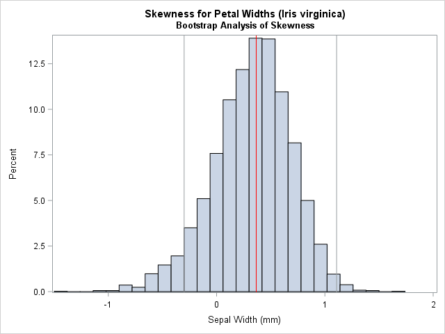
This section shows how to call the %BOOT macro. The example was previously analyzed in an article that shows how to compute a bootstrap percentile confidence interval in SAS. The statistic of interest is the skewness of the SepalWidth variable for 50 iris flowers of the species Iris virginica. The following SAS statements define the sample data and compute the skewness statistic on the original data.

%include "C:\Temp\jackboot.sas";         /* define the %BOOT and %BOOTCI macros */
 
data sample(keep=x);                     /* data are sepal widths for 50 Iris virginica flowers */
   set Sashelp.Iris(where=(Species="Virginica") rename=(SepalWidth=x));
run;
 
/* compute value of the statistic on original data: Skewness = 0.366 */
title 'Skewness for Petal Widths (Iris virginica)';
proc means data=sample nolabels skewness;
   var x;
   output out=SkewOut skew=Skewness;   /* three output variables: _type_ _freq_ and Skewness */
run;

The skewness statistic (not shown) is 0.366. The call to PROC MEANS is not necessary, but it shows how to create an output data set (SkewOut) that contains the Skewness statistic. By default, the %BOOT macro will analyze all numeric variables in the output data set, so the next step defines the %ANALYZE macro and uses the DROP= data set option to omit some unimportant variables that PROC MEANS automatically generates.

When you define the %ANALYZE macro, be sure to use the NOPRINT option or otherwise suppress ODS output during the bootstrap process. Include the %BYSTMT macro, which will tell the %BOOT macro to use a BY statement to efficiently implement the bootstrap analysis. The %ANALYZE macro is basically the same as the previous call to PROC MEANS, except for the addition of the NOPRINT, %BYSTMT, and DROP= options:

%macro analyze(data=,out=);
   proc means noprint data=&data;   
      %bystmt;
      var x;
      output out=&out(drop=_type_ _freq_) skew=Skewness;
   run;
%mend;

Although the DROP= statement is not essential, it reduces the size of the data that are read and written during the bootstrap analysis. Do NOT use a KEEP= statement in the %ANALYZE macro because the %BOOT macro will generate several other variables (called _SAMPLE_ and _OBS_) as part of the resampling process.

You can now use the %BOOT macro to generate bootstrap samples and compute basic descriptive statistics about the bootstrap distribution:

/* creates GootData, BootDist, and BootStat data sets */
title2 'Bootstrap Analysis of Skewness';
%boot(data=sample,       /* data set that contains the original data */
      samples=5000,      /* number of bootstrap samples */
      random=12345,      /* random number seed for resampling */
      chart=0,           /* do not display the old PROC CHART histograms */
      stat=Skewness,     /* list of output variables to analyze (default=_NUMERIC_) */
      alpha=0.05,        /* significance level for CI (default=0.05) */
      print=1);          /* print descriptive stats (default=1)*/
 
proc print data=bootstat noobs;  /* or use LABEL option to get labels as column headers */
   id method n;
   var value bootmean bias stderr biasco alcl aucl;
run;

I recommend that you specify the first four options. The last three options are shown in case you want to override their default values. Although the %BOOT macro prints a table of descriptive statistics, the table contains 14 columns and is very wide. To shorten the output, I used PROC PRINT to display the most important results. The table shows the estimate of the skewness statistic on the original data (VALUE), the mean of the bootstrap distribution (BOOTMEAN), the estimate for the standard error of the statistic (STDERR), and lower and upper confidence limits (ALCL and AUCL) for an approximate confidence interval under the assumption that the statistic is normally distributed. (The limits are b ± z_1-α * stderr, where z_1-α is the (1 - α)th normal quantile and b = value - bias is a bias-corrected estimate.)

The data for the bootstrap distribution is in the BootDist data set, so you can use PROC SGPLOT to display a histogram of the bootstrap statistics. I like to assign some of the descriptive statistics into macro variables so that I can display them on the histogram, as follows:

/* OPTIONAL: Store bootstrap statistic in a macro variable */
proc sql noprint;
select value, alcl,     aucl 
 into :Stat, :LowerCL, :UpperCL
 from BootStat;
quit;
 
proc sgplot data=BootDist;      /* <== this data set contains the bootstrap distribution */
   histogram Skewness;
   refline &Stat / axis=x lineattrs=(color=red);
   refline &LowerCL &UpperCL / axis=x;
run;

An example of calling the %BOOTCI macro

The %BOOTCI macro enables you to compute several confidence intervals (CIs) for the statistic that you are bootstrapping. The following statements display a percentile-based CI and a bias-adjusted and corrected CI.

title2 'Percentile-Based Confidence Interval';
%bootci(PCTL);    /* creates BootCI data set for Pctl CI */

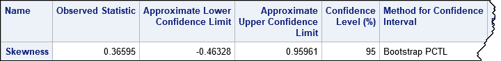
The percentile-based CI is about the same width as the normal-based CI, but it is shifted to the left. The default output from the %BOOTCI macro is very wide, so sometimes I prefer to use the PRINT=0 option to suppress the output. The estimates are written to a data set named BootCI, so it is easy to use PROC PRINT to display only the statistics that you want to see, as shown in the following call that computes a bias-corrected and adjusted interval estimate:

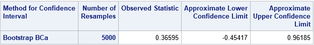
title2 'Bias-Adjusted and Corrected Bootstrap Confidence Interval';
%bootci(BCa, print=0);       /* creates BootCI data set for BCa CI */
proc print data=BootCI noobs label;
   id method n;
   var value alcl aucl;
run;

Notice that each call to the %BOOTCI macro creates a data set named BootCI. In particular, the second call overwrites the data set that was created by the first call. If you want to compare the estimates, be sure to make a copy of the first BootCI data set before you overwrite it.

The %ALLCI macro

If you want to compare multiple CIs, you can use the %ALLCI macro, which computes multiple definitions of the CIs and concatenates them into a data set named AllCI, as shown by the following:

title2 'Comparison of Bootstrap Confidence Intervals';
%allci(print=0); 
proc print data=AllCI(drop=_LABEL_) noobs label;
   id method n;
   var value alcl aucl;
run;

The output (not shown) contains interval estimates for five bootstrap CIs and a jackknife CI.

Be aware the when you run the %ALLCI macro you will see several warnings in the SAS log, such as the following:

WARNING: Variable _lo was not found on DATA file.
WARNING: Variable bootmean was not found on BASE file. The variable will
         not be added to the BASE file.

These warnings are coming from PROC APPEND and can be ignored. To suppress these warnings, you can edit the jackboot.sas file, search for the word 'force' on the PROC APPEND statements, and add the NOWARN option to those PROC APPEND statements. For example:
proc append data=bootci&keep base=ALLCI force nowarn; run;

Pros and cons of using the %BOOT macro

The %BOOT, %BOOTCI, and %ALLCI macros can be a time-saver when you want to perform a basic bootstrap in SAS. However, in my opinion, they are not a substitute for understanding how to implement a bootstrap computation manually in SAS. Here are a few advantages and disadvantages of the macros:

• Advantage: The macros encapsulate the tedious steps of the bootstrap analysis.
• Advantage: The macros generate SAS data sets that you can use for additional analyses or for graphing the results.
• Advantage: The macros handle the most common sampling schemes such as simple uniform sampling (with replacement), balanced bootstrap sampling, and residual sampling in regression models.
• Advantage: The %BOOTCI macro supports many popular confidence intervals for parameters.
• Disadvantage: The macros do not provide the same flexibility as writing your own analysis. For example, the macros do not support the stratified resampling scheme that is used for a bootstrap analysis of the difference of means in a t test.
• Disadvantage: There are only a few examples of using the macros. When I first used them, I made several mistakes and had to look at the underlying source code to understand what the macros were doing.

Summary

The %BOOT and %BOOTCI macros provide a convenient way to perform simple bootstrap analyses in SAS. The macros support several common resampling schemes and estimates for confidence intervals. Although the macros are not a replacement for understanding how to program a general, efficient, bootstrap analysis, they can be a useful tool for data analysts who want compact code to create a bootstrap analysis in SAS.