A previous article provides an example of using the BOOTSTRAP statement in PROC TTEST to compute bootstrap estimates of statistics in a two-sample t test. The BOOTSTRAP statement is new in SAS/STAT 14.3 (SAS 9.4M5). However, you can perform the same bootstrap analysis in earlier releases of SAS by using procedures in Base SAS and SAS/STAT. This article gives an example of how to bootstrap in SAS.

The main steps of the bootstrap method in SAS

A previous article describes how to construct a bootstrap confidence interval in SAS. The major steps of a bootstrap analysis follow:

1. Compute the statistic of interest for the original data
2. Resample B times (with replacement) from the data to form B bootstrap samples. The resampling process should respect the structure of the analysis and the null hypothesis. In SAS it is most efficient to use the DATA step or PROC SURVEYSELECT to put all B random bootstrap samples into a single data set.
3. Use BY-group processing to compute the statistic of interest on each bootstrap sample. The BY-group approach is much faster than using macro loops. The union of the statistic is the bootstrap distribution, which approximates the sampling distribution of the statistic under the null hypothesis.
4. Use the bootstrap distribution to obtain bootstrap estimates of bias, standard errors, and confidence intervals.

Compute the statistic of interest

This article uses the same bootstrap example as the previous article. The following SAS DATA step subsets the Sashelp.Cars data to create a data set that contains two groups: SUV" and "Sedan". There are 60 SUVs and 262 sedans. The statistic of interest is the difference of means between the two groups. A call to PROC TTEST computes the difference between group means for the data:

data Sample;    /* create the sample data. The two groups are "SUV" and "Sedan" */
set Sashelp.Cars(keep=Type MPG_City);
if Type in ('Sedan' 'SUV');
run;
 
/* 1. Compute statistic (difference of means) for data */
proc ttest data=Sample;
   class Type;
   var MPG_City;
   ods output Statistics=SampleStats;   /* save statistic in SAS data set */
run;
 
/* 1b. OPTIONAL: Store sample statistic in a macro variable for later use */
proc sql noprint;
select Mean into :Statistic
       from SampleStats where Method="Satterthwaite";
quit;
%put &=Statistic;

STATISTIC= -4.9840

The point estimate for the difference of means between groups is -4.98. The TTEST procedure produces a graph (not shown) that indicates that the MPG_City variable is moderately skewed for the "Sedan" group. Therefore you might question the usefulness of the classical parametric estimates for the standard error and confidence interval for the difference of means. The following bootstrap analysis provides a nonparametric estimate about the accuracy of the difference of means.

Resample from the data

For many resampling schemes, PROC SURVEYSELECT is the simplest way to generate bootstrap samples. The documentation for PROC TTEST states, "In a bootstrap for a two-sample design, random draws of size n1 and n2 are taken with replacement from the first and second groups, respectively, and combined to produce a single bootstrap sample." One way to carry out this sampling scheme is to use the STRATA statement in PROC SURVEYSELECT to sample (with replacement) from the "SUV" and "Sedan" groups. To perform stratified sampling, sort the data by the STRATA variable. The following statements sort the data and generate 10,000 bootstrap samples by drawing random samples (with replacement) from each group:

/* 2. Sample with replacement from each stratum. First sort by the STRATA variable. */
proc sort data=Sample; by Type; run;
 
/* Then perform stratified sampling with replacement */
proc surveyselect data=Sample out=BootSamples noprint seed=123 
                  method=urs              /* with replacement */
                  /* OUTHITS */           /* use OUTHITS option when you do not want a frequency variable */
                  samprate=1 reps=10000;  /* 10,000 resamples */
   strata Type;   /* sample N1 from first group and N2 from second */
run;

The BootSamples data set contains 10,000 random resamples. Each sample contains 60 SUVs and 262 sedans, just like the original data. The BootSamples data contains a variable named NumberHits that contains the frequency with which each original observation appears in the resample. If you prefer to use duplicated observations, specify the OUTHITS option in the PROC SURVEYSELECT statement. The different samples are identified by the values of the Replicate variable.

BY-group analysis of bootstrap samples

Recall that a BY-group analysis is an efficient way to process 10,000 bootstrap samples. Recall also that it is efficient to suppress output when you perform a large BY-group analysis. The following macros encapsulate the commands that suppress ODS objects prior to a simulation or bootstrap analysis and then permit the objects to appear after the analysis is complete:

/* Define useful macros */
%macro ODSOff(); /* Call prior to BY-group processing */
ods graphics off;  ods exclude all;  ods noresults;
%mend;
 
%macro ODSOn(); /* Call after BY-group processing */
ods graphics on;  ods exclude none;  ods results;
%mend;

With these definitions, the following call to PROC TTEST computes the Satterthwaite test statistic for each bootstrap sample. Notice that you need to sort the data by the Replicate variable because the BootSamples data are ordered by the values of the Type variable. Note also that the NumberHits variable is used as a FREQ variable.

/* 3. Compute statistics */
proc sort data = BootSamples; by Replicate Type; run;
 
%ODSOff                          /* suppress output */
proc ttest data=BootSamples;
   by Replicate;
   class Type;
   var MPG_City;
   freq NumberHits;              /* Use FREQ variable in analysis (or use OUTHITS option) */
   ods output ConfLimits=BootDist(where=(method="Satterthwaite")
              keep=Replicate Variable Class Method Mean rename=(Mean=DiffMeans)); 
run; 
%ODSOn                           /* enable output   */

Obtain estimates from the bootstrap distribution

At this point in the bootstrap example, the data set BootDist contains the bootstrap distribution in the variable DiffMeans. You can use this variable to compute various bootstrap statistics. For example, the bootstrap estimate of the standard error is the standard deviation of the DiffMeans variable. The estimate of bias is the difference between the mean of the bootstrap estimates and the original statistic. The percentiles of the DiffMeans variable can be used to construct a confidence interval. (Or you can use a different interval estimate, such as the bias-adjusted and corrected interval.) You might also want to graph the bootstrap distribution. The following statements use PROC UNIVARIATE to compute these estimates:

/* 4. Plot sampling distribution of difference of sample means. Write stats to BootStats data set */ 
proc univariate data=BootDist; /* use NOPRINT option to suppress output and graphs */
   var DiffMeans;
   histogram DiffMeans;      /* OPTIONAL */
   output out=BootStats pctlpts =2.5  97.5  pctlname=P025 P975
                  pctlpre =Mean_ mean=BootMean std=BootStdErr;
run;
 
/* use original sample statistic to compute bias */
data BootStats;
set BootStats;
Bias = BootMean - &Statistic;
label Mean_P025="Lower 95% CL"  Mean_P975="Upper 95% CL";
run;
 
proc print data=BootStats noobs; 
   var BootMean BootStdErr Bias Mean_P025 Mean_P975;
run;

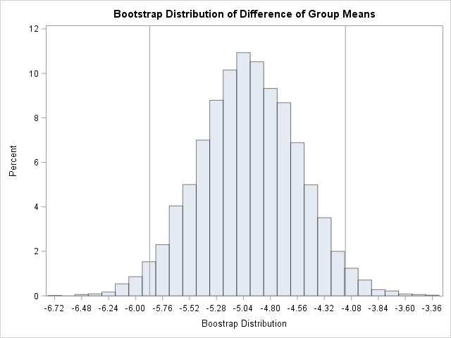
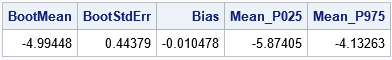
The results are shown. The bootstrap distribution appears to be normally distributed. This indicates that the bootstrap estimates will probably be similar to the classical parametric estimates. For this problem, the classical estimate of the standard error is 0.448 and a 95% confidence interval for the difference of means is [-5.87, -4.10]. In comparison, the bootstrap estimates are 0.444 and [-5.87, -4.13]. In spite of the skewness of the MPG_City variable for the "Sedan" group, the two-sample Satterthwaite t provides similar estimates regarding the accuracy of the point estimate for the difference of means. The bootstrap statistics also are similar to the statistics that you can obtain by using the BOOTSTRAP statement in PROC TTEST in SAS/STAT 14.3.

In summary, you can use Base SAS and SAS/STAT procedures to compute a bootstrap analysis of a two-sample t test. Although the "manual" bootstrap requires more programming effort than using the BOOTSTRAP statement in PROC TTEST, the example in this article generalizes to other statistics for which a built-in bootstrap option is not supported. This article also shows how to use PROC SURVEYSELECT to perform stratified sampling as part of a bootstrap analysis that involves sampling from multiple groups.