I recently showed how to compute a bootstrap percentile confidence interval in SAS. The percentile interval is a simple "first-order" interval that is formed from quantiles of the bootstrap distribution. However, it has two limitations. First, it does not use the estimate for the original data; it is based only on bootstrap resamples. Second, it does not adjust for skewness in the bootstrap distribution. The so-called bias-corrected and accelerated bootstrap interval (the BCa interval) is a second-order accurate interval that addresses these issues. This article shows how to compute the BCa bootstrap interval in SAS. You can download the complete SAS program that implements the BCa computation.
As in the previous article, let's bootstrap the skewness statistic for the petal widths of 50 randomly selected flowers of the species Iris setosa. The following statements create a data set called SAMPLE and the rename the variable to analyze to 'X', which is analyzed by the rest of the program:
data sample; set sashelp.Iris; /* <== load your data here */ where species = "Setosa"; rename PetalWidth=x; /* <== rename the analyzes variable to 'x' */ run; |
BCa interval: The main ideas
The main advantage to the BCa interval is that it corrects for bias and skewness in the distribution of bootstrap estimates. The BCa interval requires that you estimate two parameters. The bias-correction parameter, z0, is related to the proportion of bootstrap estimates that are less than the observed statistic. The acceleration parameter, a, is proportional to the skewness of the bootstrap distribution. You can use the jackknife method to estimate the acceleration parameter.
Assume that the data are independent and identically distributed. Suppose that you have already computed the original statistic and a large number of bootstrap estimates, as shown in the previous article. To compute a BCa confidence interval, you estimate z0 and a and use them to adjust the endpoints of the percentile confidence interval (CI). If the bootstrap distribution is positively skewed, the CI is adjusted to the right. If the bootstrap distribution is negatively skewed, the CI is adjusted to the left.
Estimate the bias correction and acceleration
The mathematical details of the BCa adjustment are provided in Chernick and LaBudde (2011) and Davison and Hinkley (1997). My computations were inspired by Appendix D of Martinez and Martinez (2001). To make the presentation simpler, the program analyzes only univariate data.
The bias correction factor is related to the proportion of bootstrap estimates that are less than the observed statistic. The acceleration parameter is proportional to the skewness of the bootstrap distribution. You can use the jackknife method to estimate the acceleration parameter. The following SAS/IML modules encapsulate the necessary computations. As described in the jackknife article, the function 'JackSampMat' returns a matrix whose columns contain the jackknife samples and the function 'EvalStat' evaluates the statistic on each column of a matrix.
proc iml; load module=(JackSampMat); /* load helper function */ /* compute bias-correction factor from the proportion of bootstrap estimates that are less than the observed estimate */ start bootBC(bootEst, Est); B = ncol(bootEst)*nrow(bootEst); /* number of bootstrap samples */ propLess = sum(bootEst < Est)/B; /* proportion of replicates less than observed stat */ z0 = quantile("normal", propLess); /* bias correction */ return z0; finish; /* compute acceleration factor, which is related to the skewness of bootstrap estimates. Use jackknife replicates to estimate. */ start bootAccel(x); M = JackSampMat(x); /* each column is jackknife sample */ jStat = EvalStat(M); /* row vector of jackknife replicates */ jackEst = mean(jStat`); /* jackknife estimate */ num = sum( (jackEst-jStat)##3 ); den = sum( (jackEst-jStat)##2 ); ahat = num / (6*den##(3/2)); /* ahat based on jackknife ==> not random */ return ahat; finish; |
Compute the BCa confidence interval
With those helper functions defined, you can compute the BCa confidence interval. The following SAS/IML statements read the data, generate the bootstrap samples, compute the bootstrap distribution of estimates, and compute the 95% BCa confidence interval:
/* Input: matrix where each column of X is a bootstrap sample. Return a row vector of statistics, one for each column. */ start EvalStat(M); return skewness(M); /* <== put your computation here */ finish; alpha = 0.05; B = 5000; /* B = number of bootstrap samples */ use sample; read all var "x"; close; /* read univariate data into x */ call randseed(1234567); Est = EvalStat(x); /* 1. compute observed statistic */ s = sample(x, B // nrow(x)); /* 2. generate many bootstrap samples (N x B matrix) */ bStat = T( EvalStat(s) ); /* 3. compute the statistic for each bootstrap sample */ bootEst = mean(bStat); /* 4. summarize bootstrap distrib, such as mean */ z0 = bootBC(bStat, Est); /* 5. bias-correction factor */ ahat = bootAccel(x); /* 6. ahat = acceleration of std error */ print z0 ahat; /* 7. adjust quantiles for 100*(1-alpha)% bootstrap BCa interval */ zL = z0 + quantile("normal", alpha/2); alpha1 = cdf("normal", z0 + zL / (1-ahat*zL)); zU = z0 + quantile("normal", 1-alpha/2); alpha2 = cdf("normal", z0 + zU / (1-ahat*zU)); call qntl(CI, bStat, alpha1//alpha2); /* BCa interval */ R = Est || BootEst || CI`; /* combine results for printing */ print R[c={"Obs" "BootEst" "LowerCL" "UpperCL"} format=8.4 L="95% Bootstrap Bias-Corrected CI (BCa)"]; |
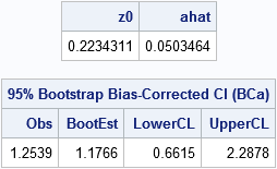
The BCa interval is [0.66, 2.29]. For comparison, the bootstrap percentile CI for the bootstrap distribution, which was computed in the previous bootstrap article, is [0.49, 1.96].
Notice that by using the bootBC and bootAccel helper functions, the program is compact and easy to read. One of the advantages of the SAS/IML language is the ease with which you can define user-defined functions that encapsulate sub-computations.
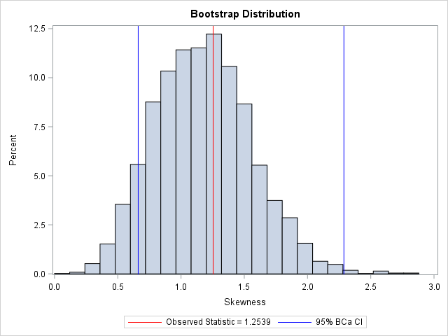
You can visualize the analysis by plotting the bootstrap distribution overlaid with the observed statistic and the 95% BCa confidence interval. Notice that the BCa interval is not symmetric about the bootstrap estimate. Compared to the bootstrap percentile interval (see the previous article), the BCa interval is shifted to the right.
There is another second-order method that is related to the BCa interval. It is called the ABC method and it uses an analytical expression to approximate the endpoints of the BCa interval. See p. 214 of Davison and Hinkley (1997).
In summary, bootstrap computations in the SAS/IML language can be very compact. By writing and re-using helper functions, you can encapsulate some of the tedious calculations into a high-level function, which makes the resulting program easier to read. For univariate data, you can often implement bootstrap computations without writing any loops by using the matrix-vector nature of the SAS/IML language.
If you do not have access to SAS/IML software or if the statistic that you want to bootstrap is produced by a SAS procedure, you can use SAS-supplied macros (%BOOT, %JACK,...) for bootstrapping. The macros include the %BOOTCI macro, which supports the percentile interval, the BCa interval, and others. For further reading, the web page for the macros includes a comparison of the CI methods.

36 Comments
Hi Rick,
Is it possible that the observed statistic is outside of the BCa? I get this for my results, and fear something is wrong.
Yes, that can happen, especially for a nonrobust statistic and outliers in the data. The confidence interval is an interval for the PARAMETER, but there is no reason why the observed statistic has to be close to the parameter. Suppose you have 999 observations that are N(0,1) and one observation that equals 10,000. The observed mean will be about 10, yet most of the bootstrap resamples will give an estimate of the mean that is close to 0. The 95% bootstrap CI will not contain 10, which is the observed mean.
Thank you for answering!
If the BCa does not cover the observed statistic (say, stat = 0.35), could I still interpret a BCa of [0.40, 0.90] to say that the statistic is significantly different from zero?
What if also the estimated mean and median of the bootstrap resamples are outside of the BCa?
All the best!
I suggest that you consult one of the references in the article, which has more details than this blog post. If you are still confused you can ask these questions on a statistical discussion forum such as stackexchange.com.
A confidence interval is a statement about the likely value of the underlying parameter, given the data. The interval [0.4, 0.9] indicates that the underlying parameter is not likely to be 0. In general, confidence intervals and significance tests say the same thing: the (1-alpha)% CI does not contain 0 iff the statistic is significantly different from 0 at the alpha significance level. So, yes, I think your statement is correct.
The bias correction factor is the estimate of the difference between the median of the bootstrap replicates and the observed statistic, in normal units (Martinez and Martinez, 2001, p. 249). Thus I would expect the median to be inside the BCa interval. I don't know about the mean. If neither is inside the CI, your program might be incorrect. Rerun it on N(0,1) data to see if the results make sense.
Thanks!
HI,
A great article about BCa method.
I have a question: when to use BCa to correct the result of bootstrap percentile intervals? Thanks!
That is a good (but difficult) question. Briefly, I use the BCa when I graph the sampling distribution and see a skewed distribution. For a more complete answer see the SAS Note about the %BOOT macro and read the section that begins "There is considerable controversy concerning the use of bootstrap confidence intervals."
Thanks for a very clear explanation of the BCa method! I have two questions regarding "the skewness of bootstrap estimates":
1. Is it possible to use replace the jackknife estimates (from JackSampMat(x)) by the bootstrap estimates (bootEst)?
2. The expressions for num and den in your code result in different values than standard skewness functions. Isn't skewness computed by using:
num = mean( (jStat-JackEst)**3)
den = mean( (jStat-JackEst)**2) ?
1. The jackknife estimate is deterministic. It depends only on the data, not on any random process. I suspect a reason to use the jackknife is to reduce the standard error of the BCa estimate.
2. The acceleration factor is RELATED to the skewness, but the formula is not the same.
Hi Rick,
Great job! Thank you for sharing this wonderful piece of code. I have been looking for some similar code in SAS for a while.
I'm doing a multivariable analysis and using 1,000-iteration bootstrap to calculate 95% CIs. My sample has n=10,000. Therefore, the jackknife procedure to calculate the acceleration takes substantially more time that the bootstrapping it self. Is there a more efficient way to calculate or approximate the acceleration from either the original distribution of x in your example, or from the distribution of bootstrap samples?
Overall, my analysis takes more than an hour to run for only 1 estimate. Since I need to do jackknife to calculate the acceleration, I may just use jackknife to calculate the 95%CI, and at least I save the time of the bootstrapping.
Thank you,
Sincerely,
I suspect you don't need to use the BCa at all. You do not say what statistic you are computing, but for n=10,000 you can probably use asymptotic formulas (when they exist) for the CIs instead of the bootstrap. If you don't have asymptotic formulas, it could still be the case that the Central Limit Theorem applies and your bootstrap distribution is approximately normal. If so, you don't need the BCa adjustment. When the bias=0 and the acceleration=0, then the BCa interval reduces to the bootstrap percentile interval.
Lastly, consider drawing a random sample of a smaller size (such as n=2500?) and running the BCa algorithm on the reduced sample. If the BCa and the percentile intervals are close, then you probably don't need the BCa.
Hi Rick, I am karthik and i work in Pharmaceutical industry. we use Bootstrap approach for Invitro dissolution comparison of Dissolution profile.We have SAS JMP software with us, however we donot have much expertise in SAS script. I will be glad if you can help us on this.
For JMP questions, you can post to the JMP Community. For SAS questions, post to the SAS Statistical Community. Each community is filled with experts who can help you.
Hi Rick,
I'm running a simulation and a particular sample has propLess = 0 causing the IML to terminate.
What is the current wisdom for such a situation? I'm inclined to either set it to missing or 1/(B+1), etc.
I'm away from the office right now, but I think that some people use
(1 + sum(bootEst < Est))/(B+1)
with the argument that the observed statistic adds one to the numerator and denominator.
Hi Dr. Wicklin, I am working through a problem that requires bootstrapped CIs for a stratified analysis. How would I BCA correct in that context? Would running the bootstrap within a strata and implementing the bca correction from the sas macro be robust? Any insights would be appreciated.
I haven't done that exact analysis myself, so I don't have any concrete advice. You probably know that you can use PROC SURVEYSELECT to perform stratified bootstrap resampling. Since stratified sampling is independent within each strata, it seems that you should be able to correct within each strata, but I haven't written any code that does that.
I ran the The bias-corrected and accelerated (BCa) bootstrap interval on PetalLength=x. and the estimate and confidence interval I got was 1.1766 (0.6615 2.2878 ), but when I run proc means I get 2.46 (2.16, 2.76). The disagreement is substantial...can this be correct? I assumed that the BCa interval produced by the program was a CI for mean petal length, but it does not appear to be. What don't I understand? I want a CI for petal length.
Sorry, but I cannot tell what statistic you are computing. In the article, I compute estimates and CI for the SKEWNESS of PetalWidth when Species="Setosa."
The skewness of PetalLength for Species="Setosa" is 0.106. A BCa interval is [-0.8, 0.9]. PROC MEANS cannot compute the CI for skewness.
I suggest you post your question and SAS program to the Statistical Procedures community at the SAS Support Communities, which is a much better environment for discussing programming questions.
Thank you very much for the useful Bca program. May I ask if the program can also return the 95% CI of the interquartile range?
You can bootstrap any statistic, including the IQR, so, yes, you could compute the sampling distribution for the IQR. Be aware that the bootstrap distribution for quantile-based statistics might not be continuous. Some researchers prefer to use the "smooth bootstrap" for quantile-based statistics.
Thank you very much for your reply Dr. Wicklin. The additional resource you provided was very helpful.
May also I ask if you happen to know what is the keyword indicating the IQR in the BCa program? E.g. what is a keyword for IQR in the following lines of code in place of "mean"?
start EvalStat(M);
return mean(M); /******** specify statistic desired: mean or median ********/
finish;
There is not a "keyword", but the following statements will compute the IQR:
Thank you very much for your reply. I was able to compute the 95%CI of the IQR.
This may be my last question. Do you happen to know the statement to compute the Root Mean Square Error (RMSE) in Bca?
?? In this article, the EvalStat function is for bootstrapping a univariate statistic. The structure of a program that bootstraps regression statistics is different and there are two common ways to bootstrap regression statistics.
It is best to ask questions like this on the SAS Support Communities. The answer to your question is
but you will need to look at my other bootstrap articles and think about how to apply the BCa analysis to a scalar regression statistic.
Hi Rick,
I am using the "bootci" function in MatLab to compute the confidence interval around the mean of a dataset. I am using the accelerated bias-corrected percentile method to compute the 95% confidence interval around the mean and I am wondering which distribution does this method assume for the data? I tried looking for this information on Mathworks website but I could not find anything about that.
Thanks in advance fr your help.
Bootstrap methods do not assume a distribution for the data.
Hi Rick,
What are your thoughts on using the BCa for estimating CI's (assuming percentile approach) around a rare event proportion? Just general thoughts would be appreciated.
I don't see any advantage to it. Let's say that your sample is size N and there is 1 event, so the observed sample statistic is 1/N. Then the bootstrap distribution if the sample proportion is going to be a discrete distribution with values at 0, 1/N, 2/N, 3/N, 4/N, and possibly 5/N. Not many samples will have 3 or more events, so most of the probability is for 0, 1/N, and 2/N. The percentile CI will probably tell you that the CI is [0, 2/N] or [0, 3/N], and I suspect the BCa will be similar. You can run an example where N=1000 to see the actual numbers.
The issue isn't really Percentile CI vs BCa. The issue is that for a rare proportion, the bootstrap distribution is discrete because the statistic can only take on a small number of possible values.
Pingback: A simple way to bootstrap linear regression models in SAS - The DO Loop
It can happen that propLess is equal to 1. Then, z0 = quantile("normal", propLess) does not work. What should be done then?
That shouldn't happen in practice. It might be an indication that (1) Your bootstrap samples are incorrect, (2) You are bootstrapping a statistic (such as a median or maximum) that is not appropriate for bootstrapping, or (3) You need to increase the number of resamples, B.
You are correct that this can theoretically happen. If all the bootstrap statistics are less than the observed statistic, I would use (B-1)/B as an estimate of PropLess. So, in the bootBC module, you could insert the statement
if propLess=1 then propLess = (B-1)/B;
before calling the QUANTILE function.
Hi Rick,
May I ask what should I do if the bias is too large and the range of bootstrap values never contains the true value? When I apply BCa method, the upper percentile is always 100% (i.e. alpha2=1) and thus the results are bad. What would you recommend to improve on this?
Also, for bootstrap-t interval, do you think it considers the bias automatically just like BCa since it takes the z score to be bootstrap value - empirical value? Then both methods will have the same order of accuracy.
Thank you in advance!
In practice, you never know the "true value", so I cannot answer that question. However, it might be that you are trying to use the bootstrap for a statistic for which the bootstrap method is not appropriate. For example, the bootstrap does not work well for quantiles such as the median or the maximum.
In principle, there is nothing wrong with having an upper percentile equal to 100%. This could occur if you are trying to get a bootstrap CL for a proportion and the true proportion is fairly large (such as 0.9).
The bootstrap t interval is first order accurate whereas BCa is second-order accurate. I would not use the t interval unless the bootstrap distribution looks VERY normal.
HI Rick, thank you for your reply! I am testing on synthetic dataset so I have the true value from the preset true population probability distribution. This always falls outside the bound of the bootstrap values as both empirical and bootstrap will give an underestimating result. So BCa becomes worse than percentile method (where I manually add in twice the bias to correct the interval) since most of the times, its upper bound falls below the true value. Is there a way to compensate for the huge bias here?
Without knowing the details, I cannot advise. You might want to post your code to the SAS Support Communities.
It is possible that you have a mistake in your bootstrap code, which is causing the situation you report. Another possibility is that synthetic data is small and/or not representative of the population. If the observed estimate is far from the parameter value, then it could be the synthetic sample is not representative. To see if that is the problem, increase the sample size (maybe N=200 or 500?) and try again.