I previously wrote about how to compute a bootstrap confidence interval in Base SAS. As a reminder, the bootstrap method consists of the following steps:
- Compute the statistic of interest for the original data
- Resample B times from the data to form B bootstrap samples. B is usually a large number, such as B = 5000.
- Compute the statistic on each bootstrap sample. This creates the bootstrap distribution, which approximates the sampling distribution of the statistic.
- Use the bootstrap distribution to obtain bootstrap estimates such as standard errors and confidence intervals.
In my book Simulating Data with SAS, I describe efficient ways to bootstrap in the SAS/IML matrix language. Whereas the Base SAS implementation of the bootstrap requires calls to four or five procedure, the SAS/IML implementation requires only a few function calls. This article shows how to compute a bootstrap confidence interval from percentiles of the bootstrap distribution for univariate data. How to bootstrap multivariate data is discussed on p. 189 of Simulating Data with SAS.
Skewness of univariate data
Let's use the bootstrap to find a 95% confidence interval for the skewness statistic. The data are the petal widths of a sample of 50 randomly selected flowers of the species Iris setosa. The measurements (in mm) are contained in the data set Sashelp.Iris. So that you can easily generalize the code to other data, the following statements create a data set called SAMPLE and the rename the variable to analyze to 'X'. If you do the same with your data, you should be able to reuse the program by modifying only a few statements.
The following DATA step renames the data set and the analysis variable. A call to PROC UNIVARIATE graphs the data and provides a point estimate of the skewness:
data sample; set sashelp.Iris; /* <== load your data here */ where species = "Setosa"; rename PetalWidth=x; /* <== rename the analyzes variable to 'x' */ run; proc univariate data=sample; var x; histogram x; inset N Skewness (6.3) / position=NE; run; |
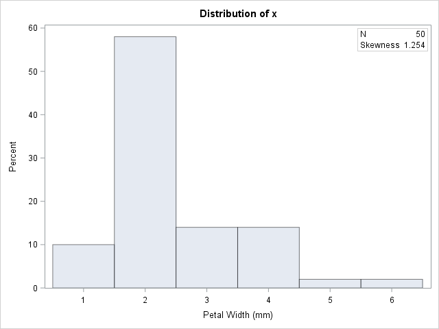
The petal widths have a highly skewed distribution, with a skewness estimate of 1.25.
A bootstrap analysis in SAS/IML
Running a bootstrap analysis in SAS/IML requires only a few lines to compute the confidence interval, but to help you generalize the problem to statistics other than the skewness, I wrote a function called EvalStat. The input argument is a matrix where each column is a bootstrap sample. The function returns a row vector of statistics, one for each column. (For the skewness statistic, the EvalStat function is a one-liner.) The EvalStat function is called twice: once on the original column vector of data and again on a matrix that contains bootstrap samples in each column. You can create the matrix by calling the SAMPLE function in SAS/IML, as follows:
/* Basic bootstrap percentile CI. The following program is based on Chapter 15 of Wicklin (2013) Simulating Data with SAS, pp 288-289. */ proc iml; /* Function to evaluate a statistic for each column of a matrix. Return a row vector of statistics, one for each column. */ start EvalStat(M); return skewness(M); /* <== put your computation here */ finish; alpha = 0.05; B = 5000; /* B = number of bootstrap samples */ use sample; read all var "x"; close; /* read univariate data into x */ call randseed(1234567); Est = EvalStat(x); /* 1. compute observed statistic */ s = sample(x, B // nrow(x)); /* 2. generate many bootstrap samples (N x B matrix) */ bStat = T( EvalStat(s) ); /* 3. compute the statistic for each bootstrap sample */ bootEst = mean(bStat); /* 4. summarize bootstrap distrib such as mean, */ SE = std(bStat); /* standard deviation, */ call qntl(CI, bStat, alpha/2 || 1-alpha/2); /* and 95% bootstrap percentile CI */ R = Est || BootEst || SE || CI`; /* combine results for printing */ print R[format=8.4 L="95% Bootstrap Pctl CI" c={"Obs" "BootEst" "StdErr" "LowerCL" "UpperCL"}]; |
The SAS/IML program for the bootstrap is very compact. It is important to keep track of the dimensions of each variable. The EST, BOOTEST, and SE variables are scalars. The S variable is a B x N matrix, where N is the sample size. The BSTAT variable is a column vector with N elements. The CI variable is a two-element column vector.
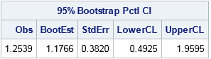
The output summarizes the bootstrap analysis. The estimate for the skewness of the observed data is 1.25. The bootstrap distribution (the skewness of the bootstrap samples) enables you to estimate three common quantities:
- The bootstrap estimate of the skewness is 1.18. This value is computed as the mean of the bootstrap distribution.
- The bootstrap estimate of the standard error of the skewness is 0.38. This value is computed as the standard deviation of the bootstrap distribution.
- The bootstrap percentile 95% confidence interval is computed as the central 95% of the bootstrap estimates, which is the interval [0.49, 1.96].
It is important to realize that these estimate will vary slightly if you use different random-number seeds or a different number of bootstrap iterations (B).
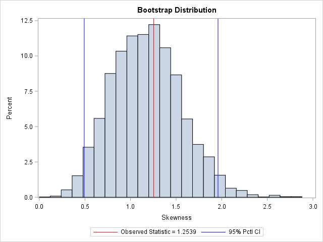
You can visualize the bootstrap distribution by drawing a histogram of the bootstrap estimates. You can overlay the original estimate (or the bootstrap estimate) and the endpoints of the confidence interval, as shown below.
In summary, you can implement the bootstrap method in the SAS/IML language very compactly. You can use the bootstrap distribution to estimate the parameter and standard error. The bootstrap percentile method, which is based on quantiles of the bootstrap distribution, is a simple way to obtain a confidence interval for a parameter. You can download the full SAS program that implements this analysis.

10 Comments
This is excellent code for anyone who might want to implement the bootstrap for data which can be assumed to be IID (independent, identically distributed). However, there are situations where the smallest unit of observation does not meet the assumption of IID. Specifically, if one is presented with data where observations are obtained from random sampling within some sort of cluster and the clusters themselves are selected at random from some larger population, then the observations across clusters are not IID.
Suppose, for instance, that one has a study where worksites are randomized to some sort of intervention program (say, a dietary modification program). The independent unit of observation is the worksite. The success of the intervention is determined based on measurements collected from individuals within worksites. Across the entire experiment, individual responses are not IID. Worksites are the independent units, and a proper bootstrap implementation for this type of study would be to sample from worksites. The code offered here would not be sufficient for such an application.
I just wanted to offer this one word of caution to an otherwise excellent presentation.
Thanks, Dale, for the kind words and the clarification. I agree completely. A guiding principal in bootstrap computations is that the resampling scheme should mimic the original sampling scheme.
Pingback: The bias-corrected and accelerated (BCa) bootstrap interval - The DO Loop
thank for sharing the article.
s = sample(x, B // nrow(x)); The S matrix is a N xB matrix, where B is the sample size. so before we use the module of EvalStat ,we may transpose the S matrix and The SKEWNESS function returns the sample of size skewness for each column of a matrix.
the BOOTEST is more near EST.
Thanks for writing. The program in the post is correct. The N x B matrix, s, is sent to the EvalStat module, which computes the skewness of each column. The function returns the B statistics from the B bootstrap samples as a 1 x B vector.
thank you ,i learn from your article,i write code as follows,but in the section of bootstrap ,there error (EXECUTION)invalid subscript or subscript out of.......
proc iml;
x = repeat({8.8,8.9,9.0,9.1,9.2,9.3,9.4,9.5,9.6,9.7,9.8,9.9,10,10.1,10.2,10.3},{1,2,1,3,11,
11,8,16,16,26,8,7,3,2,3,2})`;
start func(x);
call sort(x);
n = nrow(x);
median = median(x);
MAD = mad(x);
s = MAD/0.6745;
*---------------------------------------------------------------------------------------------------;
*cal sbt[205.6];
ui = (x-median)/(205.7*s);
flag = (ui>-1 & ui<1);
if sum(flag) -1 & ui<1);
if sum(flag) = 0.0001);
iter = iter +1;
Tbiold = Tbinew;
ui = (x-Tbi)/(c*MAD/0.6745);
if loc(ui1) then
ui[loc(ui 1)] = 1;
else ui = ui;
wi = (1-ui##2)##2;
Tbinew = (t(wi)*x)/(sum(wi));
epsilon = abs(Tbinew - Tbiold);
end;
*------------------------------------------------------------------------------------------------------;
*cal St3;
ui = (x- Tbi)/(3.7*Sbi3);
flag = (ui>-1 & ui<1);
if sum(flag) < n then
ui = ui[loc(flag)=1];
else if sum(flag)= n then
ui= ui;
ui_square = ui##2;
St3 = 3.7*Sbi3*sqrt((t(ui_square)*((1-ui_square)##4))/((t(1-ui_square)*(1-5#ui_square))*(max(1,-1+t(1-ui_square)*(1-5#ui_square)))));
tstatistic = tinv((1-(1-0.95)/2),n-1);
margin = tstatistic*sqrt(Sbi205##2 + St3##2);
ci = j(1,2,.);
ci[1] = Tbi - margin;
ci[2] = Tbi + margin;
return(ci);
finish;
*----------------------------------------------------------------------------------------------------------------------;
est = func(x);
print est;
*-----------------------------------------------------------------------------------------------------------------------;
*bootstrap;
call randseed(123);
B = 1000;
s = sample(x,B//nrow(x));
free ci;
do i = 1 to B;
B = func(s[,i]);
Bci = Bci//B;
end;
quit;
Your code was mangled when you pasted it into the comments. Try posting your question and program to the SAS Support Communities (SAS/IML Forum).
thank you
Dear Expert:
When I performed one bootstrap procedures, the final result should be n=200 meanr=0.61076 and std=0.096866. However I copied the SAS codes and the real result is n=1, meanr=0.6 and std is missing. Could you take those SAS codes and give some guidance to revise it? Thanks! I enclose the following SAS codes:
data a;
%let replicate =200; *replicate=200, the number of repeated samples;
%let unit =5; *unit=the number of original sample size (number of households);
Proc plan seed=100;
Factors replicate=&replicate ordered unit=&unit t=1 of &unit/noprint;
Output out=a; run;
Data a;
Set a;
Do j=1 to &unit; *number of different observation;
Output; end; keep replicate t unit j;
Data a1; set a; drop unit; proc sort; by replicate j;
Data a2; set a; keep replicate j unit; proc sort; by replicate j unit;
Data a; merge a1 a2; by replicate j; proc sort; by replicate j;
Data b;
/***input data***/
Input household numpeople college@@; cards;
1 4 2 2 1 1 3 5 3 4 3 1 5 2 2
;
/***end of input data***/
Data b; set b; do i=1 to &replicate ; replicate=1 ; output;
End;
Data b ; set b; keep numpeople college replicate household j;
Do j=1 to &unit; output; end;
proc sort; by replicate j;
Data final; merge a b; by replicate j; proc sort; by replicate j; run;
Data final1; set final; if j =unit; tkeep =t; keep replicate j tkeep; proc sort; by replicate j;run;
Data final2; merge final final1; by replicate j; if tkeep =household; proc sort; by replicate; run;
Proc univariate data=final2 noprint ; var numpeople college; output out =stats sum =sumnumpeople sumcollege n =n; by replicate; run;
Data stats; set stats; r =sumcollege/sumnumpeople; run;
Proc univariate noprint; var r; output out =stats1 n =n mean =meanr std =std; run;
Data stats1; set stats1; proc print; run;
You can use the SAS Support Communities to ask programming questions and get debugging help.
When you post your code there, someone will quickly point out that you only have valid values for Replicate=1 after the first DATA FINAL step.