I've written many articles about bootstrapping in SAS, including several about bootstrapping in regression models. Many of the articles use a very general bootstrap method that can bootstrap almost any statistic that SAS can compute. The method uses PROC SURVEYSELECT to generate B bootstrap samples from the data, uses the BY statement to compute a statistic on each sample, and uses PROC UNIVARIATE to obtain a percentile-based confidence interval for the underlying parameter.

After posting an article about bootstrapping for a linear regression model, a colleague reminded me that PROC GLMSELECT provides a simple way to perform a basic bootstrap for linear regression models. Namely, you can use the MODELAVERAGE statement to obtain bootstrap estimates. This article describes how to use the MODELAVERAGE statement in PROC GLMSELECT to perform a basic bootstrap analysis for the regression coefficients and for standard fit statistics such as the R-square value.

The MODELAVERAGE statement

The MODELAVERAGE statement in PROC GLMSELECT is intended for when you use variable-selection methods to choose effects in a linear regression model. It causes the GLMSELECT procedure to resample B times from the data (essentially, generates bootstrap samples) and performs variable selection and fitting on each resample. The MODELAVERAGE statement outputs the following information:

• A table that shows the proportion of the resamples for which each effect is chosen as being an important factor for predicting the response. Effects that are chosen for most samples are probably "real" effects as opposed to spurious effects.
• The average of the parameter estimates taken across all resamples. You can also get the median estimate for each effect and the upper and lower α/2 quantiles.
• If you use the OUTPUT statement, you also get average of the predicted means taken across all resamples. In addition to the mean, you can also get estimates of the median and the upper and lower α/2 quantiles of the predicted values.

Here is the key observation: If you use the SELECTION=NONE option on the MODEL statement in PROC GLMSELECT, then the MODELAVERAGE statement performs a bootstrap analysis for the regression coefficients and the predicted mean of the model.

The MODELAVERAGE statement for bootstrapping

Let's look closer at the MODELAVERAGE statement. The following SAS DATA steps create a sample data set (Sample) that contains a continuous response variable (Y) and a continuous explanatory variable (X):

/* choose data to analyze. Optionally, sort. */
data Sample(keep=x y);
   /* rename vars to X and Y to make roles easier to understand */
   set Sashelp.Class(rename=(Weight=Y Height=X));  
run;
/* OPTIONAL: Sort by X variable for future plotting */
proc sort data=Sample;  by X;  run;

First, let's use PROC GLMSELECT to compute the usual ordinary least squares estimates for the regression parameters. You can get the ordinary estimates by using the SELECTION=NONE option to suppress variable selection. The estimates are shown in the ParameterEstimates table:

/* Use PROC GLMSELECT for parameter estimates */
proc glmselect data=Sample seed=123;
    model Y=X / selection=none;   /* ordinary least squares estimates */
    ods select ParameterEstimates;
run;

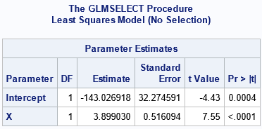
There is nothing novel about this ParameterEstimates table. These are the same estimates of the regression coefficients that you would obtain by using PROC REG or PROC GLM.

However, if you use the MODELAVERAGE statement, you get something new. Specifically, if you use the MODELAVERAGE statement and also the SELECTION=NONE on the MODEL statement, you get bootstrap estimates of the parameters. The following call to PROC GLMSELECT performs the computation. The procedure does not create a ParameterEstimates table. Instead, it produces several different tables, including the ModelAverageInfo and AvgParmEst tables:

/* Use PROC GLMSELECT for bootstrap estimates and CI */
%let NumSamples = 5000;       /* number of bootstrap resamples */ 
proc glmselect data=Sample seed=123 plots=parmdist(order=model); /* plot bootstrap distributions for coeffs */
   model Y=X / selection=none;
   modelaverage alpha=0.05 nsamples=&NumSamples; /* bootstrap estimates */
   ods select ModelAverageInfo AvgParmEst ParmDistPanel;
run;

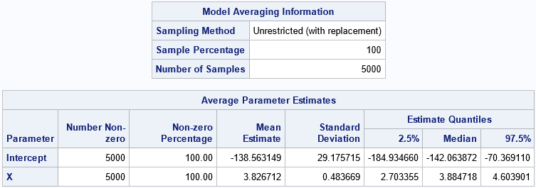
The first table is the ModelAverageInfo table. It informs you that the MODELAVERAGE statement generated B=5,000 bootstrap samples by using unrestricted random sampling (URS), which is sampling with replacement. The distribution of the 5,000 parameter estimates approximates the sampling distribution of the estimates. In the AvgParmEst table, you can see the averages and quantiles of the parameter estimates across the 5,000 samples. The following list explains the columns in the table:

• The first two columns show the number of times and the percentage that each effect appears in the selected model. Because we used the SELECTION=NONE option, all effects appear in 100% of the models.
• The "Mean Estimate" column contains the average value of the estimates for each effect. This is the bootstrap estimate of the regression parameters.
• The "Standard Deviation" column contains standard deviation of the estimates for each effect. This is the bootstrap estimate of the standard error of the regression parameters.
• The "Estimate Quantiles" columns contain selected quantiles of the estimates for each effect. The interval between the 2.5th and 97.5th percentiles is a percentile-based bootstrap estimate of the 95% confidence interval for the regression parameters. You can control the significance level by using the ALPHA= option on the MODELAVERAGE statement.

The PLOTS=PARMDIST option causes the procedure to display the distribution of the bootstrap estimates for each effect. This is shown in the following panel of graphs:

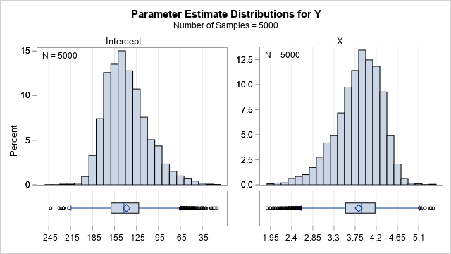
You can see that neither bootstrap distribution looks normal. The distribution of the Intercept estimates is skewed to the right; the estimates for X are skewed to the left. The next section shows how to get the 5,000 values underlying these two graphs.

Obtain the parameter estimates for each resample

The previous section shows that the MODELAVERAGE statement generates the bootstrap samples, fits the models, and provides a statistical summary of the bootstrap distribution of the estimates for the regression coefficients. The AvgParmEst table provides a 95% confidence interval for the regression coefficients, which is often the goal when an analyst uses the bootstrap. However, sometimes you might want the individual estimates from the B=5,000 bootstrap samples. You would need the individual estimates to compute more sophisticated confidence intervals, such as a bias-corrected and adjusted (BCa) confidence interval, or to estimate the covariance of the parameters.

/* use DETAILS option to get the parameter estimates for each model */
proc glmselect data=Sample seed=123;
   model Y=X / selection=none details=summary;
   modelaverage alpha=0.05 nsamples=&NumSamples
         details tables(only)=(ParmEst); 
   ods select AvgParmest;               /* display only bootstrap summary */
   ods output ParameterEstimates=PELong;/* (SLOW in 9.4!) save bootstrap distribution */
run;

The DETAILS option on the MODELAVERAGE statement results in the procedure displaying the ANOVA table, fit statistics, and parameter estimates for each of the 5,000 bootstrap samples. We do not want to see those tables, so we use the ODS SELECT statement to display only the AvgParmEst table. We use the ODS OUTPUT statement to write the 5,000 ParameterEstimate tables to a SAS data set. (Unfortunately, there was a performance bug in SAS 9.4M7, which makes this step take about 30 seconds. The bug is fixed in SAS Viya where this step takes about 1 second.)

The parameter estimates are written in long form. For many applications, it is easier to work with the estimates in wide form. The following call to PROC TRANSPOSE restructures the data into wide form. The call to PROC CORR then outputs a bootstrap estimate for the covariance of the beta parameters and plots the bootstrap distribution of each coefficient and of the joint distribution of the estimates.

/* transpose from long to wide */
proc transpose data=PELong out=PE;
   by Sample;      /* each bootstrap sample */
   id Effect;      /* Intercept, X, ... */
   var Estimate;   /* value of the estimate for the effect and sample */
run;
 
proc corr data=PE COV plots=matrix(histogram);
   var Intercept X;
run;

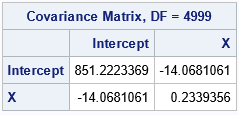
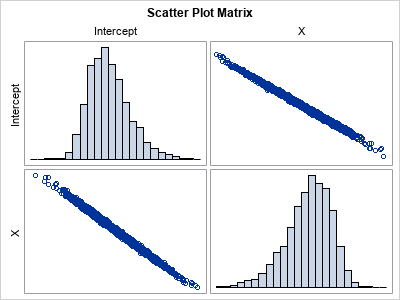
The histograms indicate the shape of the distributions of the bootstrap estimates of the model coefficients. They are the same as created earlier by using the PLOTS=PARMDIST option on the PROC GLMSELECT statement. The scatter plot indicates that the estimates are highly negatively correlated.

Other regression statistics

The DETAILS option causes the GLMSELECT procedure to display the ANOVA table, fit statistics, and parameter estimates for each of the 5,000 bootstrap samples. Consequently, you can bootstrap any of the statistics in those tables such as the R-squared or AIC statistic, which appear in the FitStatistics table. I leave the details as an exercise.

Summary

The MODELAVERAGE statement in PROC GLMSELECT enables you to perform a simple bootstrap analysis of general linear models with very little effort. By default, you obtain bootstrap standard errors and percentile-based confidence intervals for the parameter estimates. With a little more work, you can output the parameter estimates and compute other bootstrap statistics such as a BCa interval or an estimate of the covariance of the betas. You can also compute bootstrap estimates for standard statistics in the ANOVE and fit statistics tables.

This method has both advantages and disadvantages. The main advantage is that it is easy to implement and provides a simple bootstrap analysis of the regression coefficients. The main disadvantage is that you need to do additional work if you want the actual bootstrap distribution of the estimates. You also cannot perform balanced bootstrap sampling. Nevertheless, I think the MODELAVERAGE statement makes a nice addition to your toolbox of bootstrap tools.