A SAS analyst ran a linear regression model and obtained an R-square statistic for the fit. However, he wanted a confidence interval, so he posted a question to a discussion forum asking how to obtain a confidence interval for the R-square parameter. Someone suggested a formula from a textbook (Cohen, Cohen, West, & Aiken (2003), Applied multiple regression/correlation analysis for the behavioral sciences (3rd ed.), The Appendix provides the details for the formula. The formula appears to be from a paper by Olkin and Finn (1995, "Correlations Redux", Psychological Bulletin, 118(1), pp. 155-164). (Full disclosure: I do not have access to the journal, so I have not read the original paper.) I think that the formula is used by PROC GLM when you use the EFFECTSIZE option on the MODEL statement.

In general, when you receive advice on the internet, you should always scrutinize the information. In this case, the Olkin-Finn formula does not match my intuition and experience. The formula assumes that the sampling distribution of the R-square statistic is normal, but that is not correct in all cases. For simple one-variable regression, the R-square value is equal to the squared Pearson correlation between the explanatory variable, X, and the response variable, Y. Furthermore, the distribution of the correlation statistic is fairly complicated and is not normal.

To better understand the sampling distribution of the R-square statistic and when it is approximately normal, I ran a simulation study. This article presents the results of the simulation study and discusses when to use and when to avoid using the Olkin-Finn formula.

An asymptotic formula for R-square

A confidence interval is based on the sampling distribution of a statistic on random samples of data. Often (but not always) the sampling distribution depends on the distribution of the data. In order to obtain a formula, researchers often make simplifying assumptions. Common assumptions include that the data are multivariate normal, that the model is correctly specified, that the sample is very large, and so forth. The last assumption (large sample) is often used to obtain formulas that are asymptotically valid as the sample size increases. I eventually found a reference that states that the Olkin-Finn formula should not be used for small samples (degrees of freedom less than 60), so it is definitely an asymptotic formula.

By definition, the R² value is in the interval [0,1]. As we will see, the distribution of the R² statistic is highly skewed when R² is near 0 or 1. Consequently, the distribution isn't normal, and you shouldn't use the Olkin-Finn formula when R² is near 0 or 1. However, "nearness" depends on the sample size: when the sample size is large you can use the formula on a wider interval than when the sample size is small.

A simulation study for R²

The best way to understand the distribution of the R² statistic is to use a simulation. For data, I will choose a bivariate normal (BVN) sample for which the Pearson correlation is ρ. As mentioned earlier, if (X,Y) ~ BVN(0, ρ), then the regression of Y onto X has and R² value equal to the squared correlation between X and Y (=ρ²). For simplicity, I will break the simulation study into two procedure calls. First, for each value of ρ, use PROC IML to simulate 1,000 samples of size n=100 from BVN(0,ρ). Then, I will use PROC REG to run a regression on each sample and save the R² statistic into an output data set.

/* output a simulation data set: For each rho, generate 1,000
   random samples of size N for (X,Y) are bivariate normal with correlation rho */
%let NumSamples = 1000;
%let N = 100;
proc iml;
N = &N;                               /* sample size */
mu = {0 0};
Sigma = I(2);
rhoList = round( do(0, 0.9, 0.1), 0.1) || 0.95;
rho=j(N,1); SampleID=j(N,1);
create Sim var {'rho' 'SampleID' 'Y' 'X'};
do i = 1 to ncol(rhoList);
   Sigma[{2 3}] = rhoList[i];       /* set off-diagonal elements of cov matrix */
   rho[,] = rhoList[i];              
   do ID = 1 to &NumSamples;
      Z = randnormal(N, mu, Sigma);
      X = Z[,1];
      Y = Z[,2];
      SampleID[,] = ID;
      append;
  end;
end;
close;
QUIT;
 
/* run a procedure to obtain statistics for each random sample.
   In this case, obtain the R-square statistic for the regression model 
   Y = b0 + b1*X */
proc reg data=Sim noprint outest=PE;
   by rho SampleID;
   model Y = X / rsquare;  /* add R-square statistic to OUTEST= data set */
quit;

At this point, the PE data set contains a variable named _RSQ_. There is a value of _RSQ_ for each sample, and there are 1,000 samples for each ρ value. To visualize the distribution of the R-square statistic, you can use box plots, as follows:

/* plot the distribution of the R-square statistics for each rho */
proc sgplot data=PE noautolegend;
   vbox _RSQ_ / category=rho nooutliers;
   scatter x=rho y=_RSQ_ / transparency=0.8 jitter;
   yaxis grid min=0 max=1;
run;

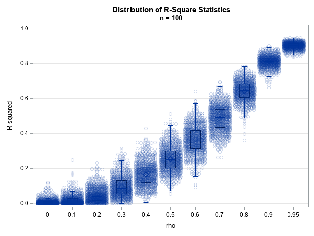
For n=100, the box plots show that the distribution of the R² statistic is skewed except when ρ is near sqrt(2) ≈ 0.7. Equivalently, ρ² is near 0.5, which is as far as ρ² can be from 0 and 1. To make the distributions easier to visualize, you can create a panel of histograms:

title "Distribution of R-Square Statistics";
title2 "n = &n";
proc sgpanel data=PE noautolegend;
   where rho in (0, 0.2, 0.4, 0.6, 0.8);
   panelby rho / rows=5 onepanel uniscale=column;
   histogram _RSQ_ / binwidth=0.02 binstart=0.01;
   density _RSQ_ / type=kernel;
   colaxis min=0 offsetmin=0.01;
run;

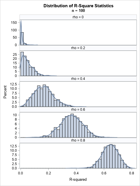
The graph demonstrates that for a small sample (n=100), the distribution of the R² statistic is not normal when R² is near 0. However, a normal approximation seems reasonable for ρ=0.6 and ρ=0.8. If you increase the sample size to, say, n=500, and rerun the program, you will notice that the R² distributions become narrower and more normal. The distribution remains skewed for extreme values of ρ.

Summary

This article reminds us that most formulas have assumptions behind them. Sometimes formulas are applicable to our data, and sometimes they are not. In this article, I use simulation to visualize the sampling distribution of the R² statistic for a simple linear regression on a small set of bivariate normal data. The simulations suggest that you should use care when using the Olkin-Finn formula for small samples. The Olkin-Finn formula is asymptotic and assumes large n. Even for large samples, the formula assumes that the sampling distribution of R-square is approximately normal, which means that you shouldn't use it when R² is near 0 or near 1.

I have no issues with using the Olkin-Finn formula for large data sets when the observed R-square statistic is not too extreme. But what should you do to obtain a confidence interval for small and mid-sized data? One possibility is to use a bootstrap analysis to estimate a confidence interval. In SAS, the GLMSELECT procedure supports the MODELAVERAGE statement, which enables you to perform a simple bootstrap analysis of many regression statistics. A bootstrap analysis does not require large samples and can correctly handle situations where the sampling distribution of R-square is skewed. In a follow-up post, I show a bootstrap analysis to estimate a confidence interval for R-square.

Appendix: The Olkin-Finn formula for a confidence interval for an R-square statistic

As discussed in this article, the Olkin-Finn formula provides an asymptotic confidence interval for R-square. The following text is from p. 88 of Cohen et al., 1988:

The text uses R₂ for the observed estimate, which is slightly confusing, but I will stick with their notation. If R² is the point estimate for a linear regression that has k parameters (not counting the intercept) and the sample has n observations, the formula approximates the sampling distribution by a normal distribution that is centered at R² and has a standard deviation that is equal to
SE = sqrt((4 R² ((1-R²)²) ((n-k-1)²)) / ((n²-1) (n + 3)))

To obtain a 100(1-α) confidence interval, you can use a normal quantile for the α level, or you can use a quantile from a t distribution with n-k-1 degrees of freedom. The following SAS DATA step shows both estimates:

/*
Online citation for formula is 
Cohen, J., Cohen, P., West, S. G., & Aiken, L. S. (2003). 
Applied multiple regression/correlation analysis for the behavioral sciences (3rd ed.)
 
The formula for the squared standard error of R^2 seems to originate from 
Olkin and Finn (1995), "Correlations Redux", Psychological Bulletin, 118(1), pp. 155-164.
 
This is an asymptotic interval, so best for  
   n - k - 1 > 60
 
For simple 1-var regression, R-sq = corr(X,Y)**2
so for rho = 0.2, R-sq = 0.04
       rho = 0.6, R-sq = 0.36
*/
%let N = 50;   /* smaller than recommended */
data AsympR2;
alpha = 0.05;  /* obtain 100*(1-alpha)% confidence interval */
n = &N;        /* sample size */
k = 1;         /* number of parameters, not including intercept */
do R2 = 0.04, 0.36;  /* observed R^2 for sample */
   SE = sqrt((4*R2*((1-R2)**2)*((n-k-1)**2))/((n**2-1)*(n + 3)));
   /* use normal quantile to estimate CI (too conservative) */
   z = quantile("Normal", 1-alpha/2);
   LCL_N = R2 - z*SE;   UCL_N = R2 + z*SE;
   /* use t quantile to estimate CI */
   t = quantile("T", 1-alpha/2, n-k-1);
   LCL_T = R2 - t*SE;   UCL_T = R2 + t*SE;
   output;
end;
run;
 
title "Asymptotic Confidence Interval (Normal Quantile)";
proc print noobs data=AsympR2; 
   var SE z LCL_N UCL_N;
   ID R2;
run;
 
title "Asymptotic Confidence Interval (t Quantile)";
proc print noobs data=AsympR2; 
   var SE t LCL_T UCL_T;
   ID R2;
run;

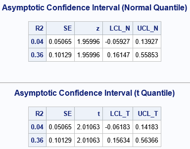
Notice that a naïve application of the Olkin-Finn formula can lead to a confidence interval (CI) that include negative values of R-square, although R-square can never be negative. You can compare the two examples to the panel of histograms that is shown earlier in this article. When ρ=0.2, the R-square value is 0.04; When ρ=0.6, the R-square value is 0.36. You can see how the Olkin-Finn CI compares to the true distribution in the histograms.