Pearson's correlation measures the linear association between two variables. Because the correlation is bounded between [-1, 1], the sampling distribution for highly correlated variables is highly skewed. Even for bivariate normal data, the skewness makes it challenging to estimate confidence intervals for the correlation, to run one-sample hypothesis tests ("Is the correlation equal to 0.5?"), and to run two-sample hypothesis tests ("Do these two samples have the same correlation?").

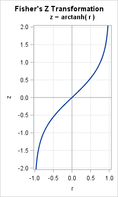
In 1921, R. A. Fisher studied the correlation of bivariate normal data and discovered a wonderful transformation (shown to the right) that converts the skewed distribution of the sample correlation (r) into a distribution that is approximately normal. Furthermore, whereas the variance of the sampling distribution of r depends on the correlation, the variance of the transformed distribution is independent of the correlation. The transformation is called Fisher's z transformation. This article describes Fisher's z transformation and shows how it transforms a skewed distribution into a normal distribution.

The distribution of the sample correlation

The following graph (click to enlarge) shows the sampling distribution of the correlation coefficient for bivariate normal samples of size 20 for four values of the population correlation, rho (ρ). You can see that the distributions are very skewed when the correlation is large in magnitude.

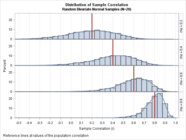
The graph was created by using simulated bivariate normal data as follows:

1. For rho=0.2, generate M random samples of size 20 from a bivariate normal distribution with correlation rho. (For this graph, M=2500.)
2. For each sample, compute the Pearson correlation.
3. Plot a histogram of the M correlations.
4. Overlay a kernel density estimate on the histogram and add a reference line to indicate the correlation in the population.
5. Repeat the process for rho=0.4, 0.6, and 0.8.

The histograms approximate the sampling distribution of the correlation coefficient (for bivariate normal samples of size 20) for the various values of the population correlation. The distributions are not simple. Notice that the variance and the skewness of the distributions depend on the value the underlying correlation (ρ) in the population.

Fisher's transformation of the correlation coefficient

Fisher sought to transform these distributions into normal distributions. He proposed the transformation f(r) = arctanh(r), which is the inverse hyperbolic tangent function. The graph of arctanh is shown at the top of this article. Fisher's transformation can also be written as (1/2)log( (1+r)/(1-r) ). This transformation is sometimes called Fisher's "z transformation" because the letter z is used to represent the transformed correlation: z = arctanh(r).

How he came up with that transformation is a mystery to me, but he was able to show that arctanh is a normalizing and variance-stabilizing transformation. That is, when r is the sample correlation for bivariate normal data and z = arctanh(r) then the following statements are true (See Fisher, Statistical Methods for Research Workers, 6th Ed, pp 199-203):

• The distribution of z is approximately normal and "tends to normality rapidly as the sample is increased" (p 201).
• The standard error of z is approximately 1/sqrt(N-3), which is independent of the value of the correlation.

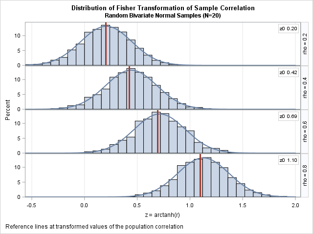
The graph to the right demonstrates these statements. The graph is similar to the preceding panel, except these histograms show the distributions of the transformed correlations z = arctanh(r). In each cell, the vertical line is drawn at the value arctanh(ρ). The curves are normal density estimates with σ = 1/sqrt(N-3), where N=20.

The two features of the transformed variables are apparent. First, the distributions are normally distributed, or, to quote Fisher, "come so close to it, even for a small sample..., that the eye cannot detect the difference" (p. 202). Second, the variance of these distributions are constant and are independent of the underlying correlation.

Fisher's transformation and confidence intervals

From the graph of the transformed variables, it is clear why Fisher's transformation is important. If you want to test some hypothesis about the correlation, the test can be conducted in the z coordinates where all distributions are normal with a known variance. Similarly, if you want to compute a confidence interval, the computation can be made in the z coordinates and the results "back transformed" by using the inverse transformation, which is r = tanh(z).

You can perform the calculations by applying the standard formulas for normal distributions (see p. 3-4 of Shen and Lu (2006)), but most statistical software provides an option to use the Fisher transformation to compute confidence intervals and to test hypotheses. In SAS, the CORR procedure supports the FISHER option to compute confidence intervals and to test hypotheses for the correlation coefficient.

The following call to PROC CORR computes a sample correlation between the length and width of petals for 50 Iris versicolor flowers. The FISHER option specifies that the output should include confidence intervals based on Fisher's transformation. The RHO0= suboption tests the null hypothesis that the correlation in the population is 0.75. (The BIASADJ= suboption turns off a bias adjustment; a discussion of the bias in the Pearson estimate will have to wait for another article.)

proc corr data=sashelp.iris fisher(rho0=0.75 biasadj=no);
   where Species='Versicolor';
   var PetalLength PetalWidth;
run;

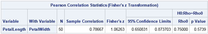
The output shows that the Pearson estimate is r=0.787. A 95% confidence interval for the correlation is [0.651, 0.874]. Notice that r is not the midpoint of that interval. In the transformed coordinates, z = arctanh(0.787) = 1.06 is the center of a symmetric confidence interval (based on a normal distribution with standard error 1/sqrt(N-3)). However, the inverse transformation (tanh) is nonlinear, and the right half-interval gets compressed more than the left half-interval.

For the hypothesis test of ρ = 0.75, the output shows that the p-value is 0.574. The data do not provide evidence to reject the hypothesis that ρ = 0.75 at the 0.05 significance level. The computations for the hypothesis test use only the transformed (z) coordinates.

Summary

This article shows that Fisher's "z transformation," which is z = arctanh(r), is a normalizing transformation for the Pearson correlation of bivariate normal samples of size N. The transformation converts the skewed and bounded sampling distribution of r into a normal distribution for z. The standard error of the transformed distribution is 1/sqrt(N-3), which does not depend on the correlation. You can perform hypothesis tests in the z coordinates. You can also form confidence intervals in the z coordinates and use the inverse transformation (r=tanh(z)) to obtain a confidence interval for ρ.

The Fisher transformation is exceptionally useful for small sample sizes because, as shown in this article, the sampling distribution of the Pearson correlation is highly skewed for small N. When N is large, the sampling distribution of the Pearson correlation is approximately normal except for extreme correlations. Although the theory behind the Fisher transformation assumes that the data are bivariate normal, in practice the Fisher transformation is useful as long as the data are not too skewed and do not contain extreme outliers.

You can download the SAS program that creates all the graphs in this article.