Convert a symmetric matrix from wide to long form

For graphing multivariate data, it is important to be able to convert the data between "wide form" (a separate column for each variable) and "long form" (which contains an indicator variable that assigns a group to each observation). If the data are numeric, the wide data can be represented as an N x p matrix. The same data in long form can be represented by two columns and Np rows, where the first column contains the data and the second column identifies that the first N rows belong to the first group, the second N rows belong to the second group, and so on. Many people have written about how to use PROC TRANSPOSE or the SAS DATA step to convert from wide form to long form and vice versa.

The conversion is slightly different for a symmetric matrix because you might want to display only the upper-triangular portion of the matrix. This article examines how to convert between a symmetric correlation matrix (wide form) and a "compressed symmetric" form that only stores the elements in the upper-triangular portion of the symmetric matrix.

Compressed symmetric storage

When the data represents a symmetric N x N matrix, you can save space by storing only half the data, such as only the upper triangular portion of the matrix. This is called compressed symmetric storage. Familiar examples of symmetric matrices include correlation, covariance, and distance matrices. For example, you can represent the 3 x 3 symmetric matrix A = {3 2 1, 2 5 0, 1 0 9} by storing only the upper triangular entries U = {3, 2, 1, 5, 0, 9}. There are N(N+1)/2 upper triangular elements. For a correlation matrix, you don't need to store the diagonal elements; you only need to store N(N-1)/2 elements.

When you run a correlation analysis by using PROC CORR in SAS, you usually get a square symmetric matrix of correlation estimates. However, if you use the FISHER option to get confidence limits for the correlation coefficients, then you get a table that shows the correlation estimates for each pair of variables. I will demonstrate this point by using the Sashelp.Iris data. To make the discussion general, I will put the variable names into a macro variable so that you can concentrate on the main ideas:

data sample;   /* use a subset of the Iris data */
   set Sashelp.Iris(where=(Species="Versicolor"));
   label PetalLength= PetalWidth= SepalLength= SepalWidth=;
run;
 
%let varNames = PetalLength PetalWidth SepalLength SepalWidth;
/* count how many variables are in the macro variable */
data _null_;
nv = countw("&varNames");
call symputx("numVars", nv);
run;
%put &=numVars;   /* for this example, numVars=4 */
 
proc corr data=sample fisher(rho0=0.7 biasadj=no) noprob outp=CorrOut;
   var &varNames;
   ods select PearsonCorr FisherPearsonCorr;
   ods output FisherPearsonCorr = FisherPCorr;
run;

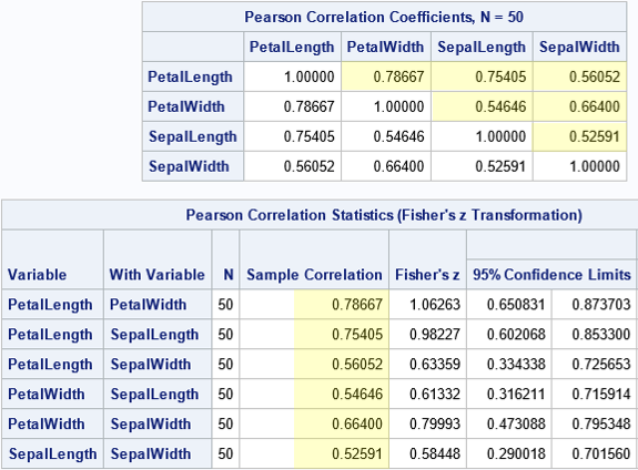
The usual square symmetric correlation matrix is shown at the top of the image. I have highlighted the elements in the strictly upper triangular portion of the matrix. By using these values, you can re-create the entire matrix. The second table is an alternative display that shows only the six pairwise correlation estimates. The arrangement in the second table can be useful for plotting the pairwise correlations in a bar chart.

It is useful to be able to convert the first table into the format of the second table. It is also useful to be able to augment the second table with row/column information so that each row of the second table is easily associated with the corresponding row and column in the first table.

Convert a symmetric table to a pairwise list

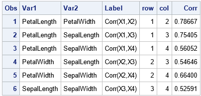
Let's use the information in the first table to list the correlations for pairs of variables, as shown in the second table. Notice that the call to PROC CORR uses the OUTP= option to write the correlation estimates to a SAS data set. You should print that data set to understand its structure; it contains more than just the correlation estimates! After you understand the structure, the following DATA step will make more sense. The main steps of the transformation are:

Create a variable named ROW that has the values 1, 2, 3, ..., N. In the following DATA step, I use the MOD function because in a subsequent article, I will use the same DATA step to perform a bootstrap computation in which the data set contains B copies of the correlation matrix.
Create a variable named COL. For each value of ROW, the COL variable loops over the values ROW+1, ROW+2, ..., N.
Put the correlation estimates into a single variable named CORR.
If desired, create a short label that identifies the two variables that produced the correlation estimate.

/* Convert correlations in the OUTP= data set from wide to long form (pairwise statistics) */
data Long;
set CorrOut(where=(_Type_="CORR") rename=(_NAME_=Var1));
length Var2 $32 Label $13;
array X[*] &varNames;
row = 1 + mod(_N_-1, &NumVars);   /* 1, 2, ..., N, 1, 2, ..., N, 1, 2, ... */
do col = row+1 to &NumVars;       /* names for columns */
   Var2 = vname(X[col]);
   Corr = X[col];
   Label = cats("Corr(X",row,",X",col,")");
   output;
end;
drop _TYPE_ &varNames;
run;
 
proc print data=Long; run;

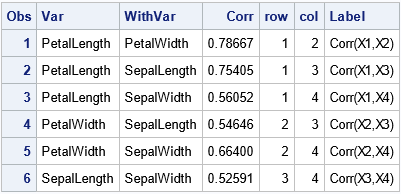
The ROW and COL variables identify the position of the correlation estimates in the upper-triangular portion of the symmetric correlation matrix. You can write a similar DATA step to convert a symmetric matrix (such as a covariance matrix) in which you also want to display the diagonal elements.

Identify the rows and columns of a pairwise list

The data for the second table is stored in the FisherPCorr data set. Although it is possible to convert the pairwise list into a dense symmetric matrix, a more useful task is to identify the rows and columns for each entry in the pairwise list, as follows:

/* Write the (row,col) info for the list of pairwise correlations in long form */
data FisherCorr;
set FisherPCorr;
retain row col 1;
if col>=&NumVars then do;
   row+1;
   col=row;
end;
col+1;
Label = cats("Corr(X",row,",X",col,")");
run;
 
proc print data=FisherCorr; 
   var Var WithVar Corr row col Label;
run;

From the ROW and COL variables, you can assemble the data into a symmetric matrix. For example, I've written about how to use the SAS/IML language to create a symmetric correlation matrix from the strictly upper-triangular estimates.

Summary

For a symmetric matrix, you can display the matrix in a wide format (an N x N matrix) or you can display the upper-triangular portion of the matrix in a single column (long format). This article shows how to use the SAS DATA step to convert a correlation matrix into a long format. By adding some additional variables, you can identify each value with a row and column in the upper-triangular portion of the symmetric matrix.

Blogs