Bootstrap predicted means by using PROC GLMSELECT

A previous article shows how to use the MODELAVERAGE statement in PROC GLMSELECT in SAS to perform a basic bootstrap analysis of the regression coefficients and fit statistics. A colleague asked whether PROC GLMSELECT can construct bootstrap confidence intervals for the predicted mean in a regression model, as described in an article about bootstrapping the predicted mean of a regression model. Yes! This article shows how to use the PROC GLMSELECT to perform a simple bootstrap analysis of the predicted mean on a scoring data set for general linear regression models.

Create data and a scoring data set

The goal of this analysis is to compute a bootstrap distribution of the predicted values at each point in the scoring data. From the distribution, you can obtain a confidence interval for the predicted mean at each point. The following SAS DATA steps create a small data set (Sample) for fitting a regression model and a second data set (ScoreData) that contains points at which to evaluate the model. These data sets are then concatenated so that you can use the "missing response trick" to score the data by using the OUTPUT statement in a regression procedure. (If you are a SAS statistical programmer, you must know this trick!)

/* choose data to analyze. Optionally, sort. */
data Sample(keep=x y);
   /* rename vars to X and Y to make roles easier to understand */
   set Sashelp.Class(rename=(Weight=Y Height=X));  
run;
/* OPTIONAL: Sort by X variable for future plotting */
proc sort data=Sample;  by X;  run;
 
/* create a scoring set */
data ScoreData;
   do X = 50 to 75 by 5;
      ScoreId + 1;
      output;
   end;
run;
/* concatenate scoring points with the data for fitting the model */
data SampleAndScore;
   set Sample ScoreData(in=S);
   IsScore = S;                /* indicator variable: 1 for scoring data; 0 for original data */
run;

Fit and score many bootstrap samples

You can use the MODELAVERAGE statement in PROC GLMSELECT to perform a basic bootstrap analysis. The following statements create B=5,000 bootstrap sample, fit the model on each, and output the predicted mean at each point in the input data set. The use of the WHERE clause in the OUTPUT statement causes the procedure to output only the predicted values at the points in the scoring data, not at the points used to fit the model.

/* Output the bootstrap mean, 2.5th pctl, and 97.5th pctl of the predicted values at each scoring point */
proc glmselect data=SampleAndScore seed=123;
    model Y=X / selection=none;                    /* specify the model */
    modelaverage alpha=0.05 nsamples=&NumSamples;  /* generate bootstrap samples */
    output out=GLSOut(where=(IsScore=1))           /* output values only for the scoring set */
           P=BootMean lower=Pctl_2_5 upper=Pctl_97_5;  /* summary statistics for distribution of predicted mean */
run;
 
proc print data=GLSOut noobs;
   var ScoreID X BootMean Pctl_2_5 Pctl_97_5;
run;

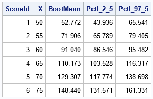
The output shows the bootstrap average and a 95% bootstrap confidence interval for the predicted mean at each point in the scoring set. I think this is a cool result. If you perform the same computations using procedures such as PROC SURVEYSELECT, PROC REG, and PROC SCORE, you must write more lines of code. You can compare this output to the output in my previous article to see that the bootstrap estimates are similar.

Obtain the bootstrap estimates for each resample

If you need the B=5,000 predicted means at each point in the scoring data, you can get them by using the SAMPLEPRED= option on the OUTPUT statement, as follows:

proc glmselect data=SampleAndScore seed=123;
    model Y=X /selection = none;
    modelaverage alpha=0.05 nsamples=&NumSamples;
    output out=GLSOut(where=(IsScore=1))  /* output values only for the scoring set */
           P=BootMean SamplePred=Pred;    /* variables are Pred1, Pred2, ... */
run;

After running these statements, the GLSOut data contains six rows (one for each value in the scoring data set) and the new variables Pred1–Pred5000. The columns contain the predicted values for the scoring data when the model is fit the 1st, 2nd, ..., 5000th bootstrap sample.

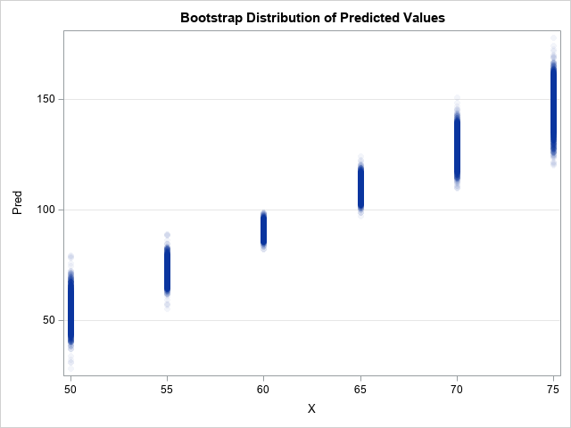
In some situations, you might want to convert the GLSOut data from wide to long format. You can use a DATA step to convert the data set to long form. You can then plot the data or compute descriptive statistics for the bootstrap distribution.

/* wide to long transpose */
data BootDist;
   set GLSOut;
   by ScoreID;
   array P[*] Pred1-Pred&NumSamples;
   do i = 1 to dim(P);
      Pred = P[i];
      output;
   end;
   keep ScoreID X Pred BootMean;
run;
 
title "Bootstrap Distribution of Predicted Values";
proc sgplot data=BootDist;
   scatter x=X y=Pred / markerattrs=(Symbol=CircleFilled) transparency=0.95;
   yaxis grid;
run;

Summary

If you use the SELECTION=NONE option on the MODEL statement in PROC GLMSELECT, you can use the MODELAVERAGE statement to perform simple bootstrap computations. A previous article shows that you can bootstrap the regression coefficients and fit statistics. This article shows that you can bootstrap the predicted means to obtain confidence intervals for the conditional mean at each point in a scoring data set.

The MODELAVERAGE statement is easy to use, but only gives simple percentile-based bootstrap confidence intervals. For more sophisticated bootstrap analyses, you can use the SAMPLEPRED= option on the OUTPUT statement to obtain the predicted mean for each bootstrap sample in the analysis.

Although it isn't shown in this article, you can also use the SAMPLEFREQ= option on the OUTPUT statement to obtain the bootstrap samples themselves. See the documentation for the SAMPLEFREQ= option.

Blogs