In ordinary least squares regression, there is an explicit formula for the confidence limit of the predicted mean. That is, for any observed value of the explanatory variables, you can create a 95% confidence interval (CI) for the predicted response. This formula assumes that the model is correctly specified and that errors in the data are independent, homogeneous, and normally distributed. In SAS, you can compute the CI by using the LCML= and UCLM= option on the OUTPUT statement in PROC REG.

Of course, not every regression model provides explicit formulas. And even for regression models that have formulas, it is not always clear whether the data satisfy the assumption of the model. Thus, the bootstrap method is an important tool to estimate these confidence intervals. This article demonstrates how to compute a bootstrap CI for the predicted response in a simple least squares model in SAS. You can estimate the CIs for every row in a set of scoring data, which specifies the values of the explanatory variables at which to evaluate the regression model. The example in this article has only one explanatory variable, but the ideas apply to models that contain multiple continuous or categorical explanatory variables.

Predicted values are statistics

It is common to use bootstrap methods to provide CIs for statistics such as the regression coefficient estimates. The predicted values of a model are also statistics. As such, they have a sampling distribution that you can estimate by using the bootstrap. From the sampling distribution, you can estimate quantities such as confidence intervals. Notice that you must specify values of the explanatory variables because you are trying to estimate the distribution of the conditional predicted mean E[Y|X]. You will get a different distribution for each value of the explanatory variables. In this article, I estimate the CIs at a set of values in a scoring data set.

Choose data and a scoring data set

The following DATA step creates an example data set with variables Y (the response variable) and X (the explanatory variable) from the Sashelp.Class data, which has 19 observations:

/* choose data to analyze. Optionally, sort. */
data Sample(keep=x y);
   /* rename vars to X and Y to make roles easier to understand */
   set Sashelp.Class(rename=(Weight=Y Height=X));  
run;
/* OPTIONAL: Sort by X variable for future plotting */
proc sort data=Sample;  by X;  run;

In addition, you can use a DATA step to creates values at which to estimate the confidence limits for the predicted mean. The following statements define a data set that contains six equally spaced values.

/* create a scoring set */
data ScoreData;
   do X = 50 to 75 by 5;
      ScoreId + 1;         /* include an ID variable */
      output;
   end;
run;

Bootstrap predicted values for a regression model

If you have never used the bootstrap in SAS before, see the article, "The Essential Guide to Bootstrapping in SAS." As discussed in the article, there are four main steps to bootstrapping:

1. Compute a statistic for the original data. For this article, the statistic is the predicted mean of the response at each value in the scoring data. (For a linear regression model, you can also request a parametric estimate of the CI of the predicted mean.)
2. Use the DATA step or PROC SURVEYSELECT to resample (with replacement) B times from the data. For efficiency, you should put all B random bootstrap samples into a single data set. This example uses case resampling to form the bootstrap samples.
3. Use BY-group processing to compute the statistic of interest on each bootstrap sample. The union of the statistic is the bootstrap distribution. Remember to turn off ODS when you run BY-group processing!
4. Use the bootstrap distribution to obtain inferential estimates. This article computes the confidence intervals for the predicted value at each observed value of the explanatory variables. It uses simple percentile-based confidence intervals.

The following SAS program carries out the first two steps of the bootstrap method:

/* 1. Compute the statistics on the original data. Estimate CLM by using the asymptotic formula.
      Concatenate the scoring data and use the "missing response trick" 
      https://blogs.sas.com/content/iml/2014/02/17/the-missing-value-trick-for-scoring-a-regression-model.html
*/
data SampleAndScore;
   set Sample ScoreData(in=S);
   IsScore = S;
run;
proc reg data=SampleAndScore plots(only)=FitPlot(nocli);
   model Y = X;
   /* output the theoretical CI for each scoring observation for later comparison */
   output out=RegOut(where=(IsScore=1)) Pred=Pred LCLM=LowerP UCLM=UpperP;
run; quit;
 
/* 2. Generate many bootstrap samples by using PROC SURVEYSELECT */
%let NumSamples = 5000;       /* number of bootstrap resamples */ 
proc surveyselect data=Sample NOPRINT seed=1
     out=BootCases(rename=(Replicate=SampleID))
     method=urs              /* resample with replacement */
     samprate=1              /* each bootstrap sample has N observations */
     /* OUTHITS                (optional) use OUTHITS option to suppress the frequency var */
     reps=&NumSamples;       /* generate NumSamples bootstrap resamples */
run;

At this point, we have two data sets:

• The RegOut data set contains the predicted mean response and the parametric CIs for each value in the scoring data. I used the OUTPUT statement and the "missing response trick" to score the data. The CIs are obtained by using a standard formula.
• The BootCases data set contains B=5,000 bootstrap samples of the data.

Step 3 requires computing the required statistics (the predicted mean at each point in the scoring data) for every bootstrap sample. There are many ways to score a regression model in SAS, but I will use the OUTEST= option in PROC REG to save the parameter estimates for each bootstrap sample and use PROC SCORE to score the models on the scoring data, as follows:

/* 3. Compute the statistics for each bootstrap sample. */
proc reg data=BootCases outest=PE noprint;    /* fit the model and save the parameter estimates for each sample */
   by SampleID;
   freq NumberHits;
   model Y = X;
run;quit;
 
proc score data=ScoreData score=PE type=parms predict /* score each model on the scoring data */
           out=BootOut(rename=(MODEL1=Pred));
   by SampleID;
   var X;
run;

The astute reader might wonder how BY processing works with PROC SCORE if the scoring data set does not contain the BY-group variable. The answer is that PROC SCORE does the natural thing: It uses the same set of scoring data for all BY groups. To remind you of this behavior, PROC SCORE displays the following note in the log:

NOTE: No BY variables are present in the DATA= data set. Each
      BY group of the SCORE= data set will be used to compute
      scores for the entire DATA= data set.

At this point, the BootOut data set contains 30,000 predicted values. There are 6 observations in the scoring data, and the predicted values are computed at each point for 5,000 bootstrap samples. In general, if you have k scoring values and use B bootstrap samples, you will get k*B rows in the BootOut data set.

Estimating the confidence intervals

You can now estimate a 95% confidence interval. The simplest estimate is to use the 2.5th and 97.5th percentiles of the predicted values at each scoring point. You can use PROC UNIVARIATE to estimate these percentiles:

/* 4. Compute the bootstrap 95% prediction CL for each row in the score data */
/* Find the 2.5th and 97.5th percentiles for the bootstrap statistics each X value */
proc univariate data=BootOut noprint;
   class ScoreID;
   var Pred;
   output out=BootCL mean=BootMean pctlpre=Pctl_ pctlpts=2.5, 97.5; 
run;

I used the CLASS statement instead of the BY statement to avoid having to sort the predicted values by the ID of the scoring data. The BootCL data set contains the bootstrap mean of the predicted values, as well as estimates of a 95% CI. The following call to PROC SGPLOT overlays the bootstrap means and CIs for the scoring data. The confidence intervals are displayed by using the HIGHLOW statement:

/* merge the REG output and the bootstrap CL */
data All;
   merge RegOut BootCl;
   by ScoreID;
run;
 
/* visualize the bootstrap mean and CLM */
title "Bootstrap CLM";
title2 "&NumSamples Bootstrap Samples";
proc sgplot data=All;
   series x=x y=Pred / legendlabel="OLS Pred" lineattrs=(color=gray);
   scatter x=x y=BootMean / legendlabel="Boot Pred" markerattrs=(symbol=X);
   highlow x=x low=Pctl_2_5 high=Pctl_97_5 / legendlabel="Boot CLM"
               lowcap=serif highcap=serif lineattrs=GraphError;
   yaxis label="Y";
run;

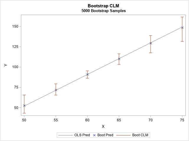
The graph visualizes the bootstrap estimates of the confidence interval for the predicted mean at the six points in the scoring data. At each X value, the bootstrap estimate of the conditional mean (marked by using an 'x' symbol) is close to the predicted mean from the original model.

Compare the bootstrap confidence intervals to theory

For most regression models, the bootstrap analysis is complete at this point. However, for the linear regression model, there is a theoretical formula for the CI of the conditional predicted mean. That means you can compare the bootstrap CIs to the theoretical CIs. I previously saved the theoretical CIs by using the LCLM= and UCLM= options on the OUTPUT statement in PROC REG. The following call to PROC SGPLOT overlays the two interval estimates.

/* visualize the bootstrap mean and CLM */
title "Compare OLS and Bootstrap CLM";
title2 "&NumSamples Bootstrap Samples";
proc sgplot data=All;
   series x=x y=Pred / legendlabel="OLS Pred" lineattrs=(color=gray);
   highlow x=x low=LowerP high=UpperP / legendlabel="OLS CLM"
               lowcap=serif highcap=serif lineattrs=GraphData1(thickness=2);
   scatter x=x y=BootMean / legendlabel="Boot Pred" markerattrs=(symbol=X);
   highlow x=x low=Pctl_2_5 high=Pctl_97_5 / legendlabel="Boot CLM"
               lowcap=serif highcap=serif lineattrs=GraphError(thickness=2);
   yaxis label="Y";
run;

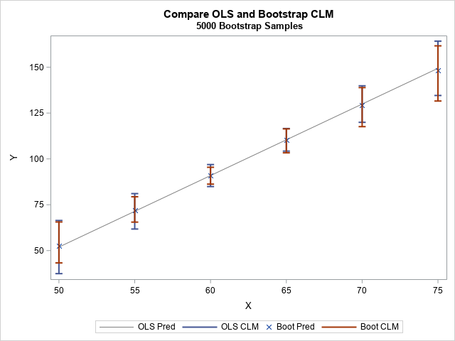
You can see that the two CI estimates are similar. The theoretical CI is symmetric about the conditional predicted mean, whereas the bootstrap CI does not have to be symmetric.

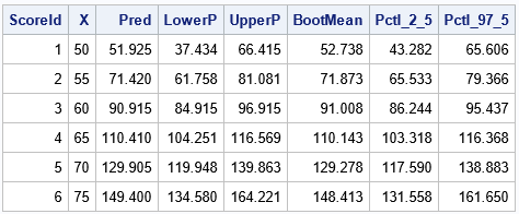
In case you want to view the actual numbers, the following table displays the theoretical estimates and the bootstrap estimates for this example at each point in the scoring set:

Summary

Let's review what we've done. We started with a regression model that predicts the mean response at some value of X, the explanatory variable. We want to know how confident we are in that prediction at X. To answer that question, we resample 5,000 times from the data, which simulates the process of collecting an additional 5,000 random samples. For each resample, we refit the model and obtain a predicted value at X. Thus, we obtain a distribution of conditional predicted values. The distribution enables us to quantify the uncertainty in the prediction by providing a confidence interval for the predicted value at X.

This example might be more complicated than other bootstrap examples that you have seen because this example bootstraps multiple values of X simultaneously. This requires fitting and scoring a regression model for each bootstrap sample. The result is a confidence interval for the predicted mean at each value in a scoring data set.