I have previously blogged about ways to perform balanced bootstrap resampling in SAS. I recently learned about an easier way: Since SAS/STAT 14.2 (SAS 9.4M4), the SURVEYSELECT procedure has supported balanced bootstrap sampling. This article reviews balanced bootstrap sampling and shows how to use the METHOD=BALBOOT option in PROC SURVEYSELECT to run a balanced bootstrap in SAS. It also addresses the question: Should the balanced bootstrap method be preferred over the traditional bootstrap?

What is the balanced bootstrap?

The traditional bootstrap method creates bootstrap samples (called resamples) by sampling with replacement from the original data, which has N observations. This is called "uniform" resampling because each observation has a uniform probability of 1/N of being selected at each step of the resampling process. Within the union of the B bootstrap samples, each observation has an expected value of appearing B times, but the actual distribution of the frequencies is multinomial.

Balanced bootstrap resampling (Davison, Hinkley, and Schechtman, 1986) is an alternative process in which each observation appears exactly B times in the union of the bootstrap samples. In SAS, you can use the METHOD=BALBOOT option in PROC SURVEYSELECT to generate balanced bootstrap samples.

How many times is each observation selected in a traditional bootstrap?

To demonstrate the difference between a traditional set of bootstrap resamples and a set of balanced bootstrap samples, consider the following 10 observations from Davison, Hinkley, and Schechtman (1986). DHS used these data to bootstrap an estimate of the sampling distribution of the sample mean. The sample size is small and the data are not normal, therefore we do not expect the sampling distribution of the mean to be normally distributed.

data Sample;
input x @@;
datalines;
9.6 10.4 13.0 15.0 16.6 17.2 17.3 21.8 24.0 33.8
;

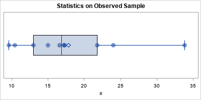
The graph shows the distribution of the data. You can use PROC MEANS to estimate the mean, standard error, and 90% confidence interval (CI) for the population mean:

title "Statistics on Observed Sample";
proc means data=Sample N Mean StdErr alpha=0.1 CLM;
   var x;
run;

The standard error and the CI estimates are based on a formula that applies when the sample is large or is normally distributed. Neither situation applies to these data. However, you can use the bootstrap method to obtain bootstrap estimates of the standard error and CI.

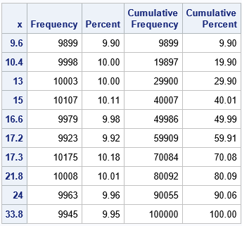
Traditional bootstrap samples are generated by sampling from the data with replacement. You can use PROC SURVEYSELECT and the METHOD=URS option to generate bootstrap samples. The following statements generate one data set that contains B=10,000 resamples of size N=10. Each sample is identified by a unique value of the SampleID variable. After generating the B=10,000 samples, you can use PROC FREQ to determine how often each observation was selected.

/* use the traditional bootstrap sampling with METHOD=URS */
%let NumSamples = 10000;     /* B = number of bootstrap resamples */
proc surveyselect data=Sample NOPRINT seed=1  /* SEED for RNG */
     method=urs              /* URS = resample with replacement */
     samprate=1              /* each bootstrap sample has N obs */
     OUTHITS                 /* do not use a frequency var */
     reps=&NumSamples(repname=SampleID)        /* generate NumSamples samples */
     out=BootSamp;
run;
 
/* overall, how often was each observation selected? */
proc freq data=BootSamp;
   tables x;
run;

The output from PROC FREQ shows that, on average, each observation is selected about B times. However, some observations are selected more often than others. One observation (9.6) was selected only 9,899 times whereas another (17.3) was selected 10,175 times. This can affect the statistics on the resamples. Overall, the value 9,6 appears less often than 17.3, so it has less influence on the bootstrap statistics. If an outlier is selected more or less often than expected, this might affect the inferences that you are trying to make.

How to run a balanced bootstrap analysis in SAS

An alternative way to generate bootstrap samples is by using a method called balanced bootstrap sampling. In balanced bootstrap sampling, each observation is selected equally often over the course of the B resamples. You can use the METHOD=BALBOOT option (and omit the SAMPRATE= option) to generate B=10,000 bootstrap resamples, as follows:

proc surveyselect data=Sample NOPRINT seed=1  /* SEED for RNG */
     method=BalBoot          /* balanced bootstrap sampling */
     OUTHITS                 /* do not use a frequency var */
     reps=&NumSamples(repname=SampleID) /* generate NumSamples samples */
     out=BalBootSamp;
run;
 
/* overall, how often was each observation selected? */
proc freq data=BalBootSamp;
   tables x;
run;

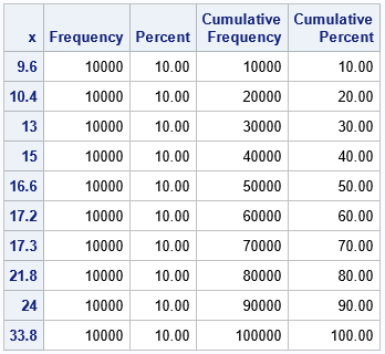
The output from PROC FREQ shows that each observation was selected a total of B times over the course of generating the B bootstrap samples. Of course, for any one observation, some resamples do not contain it, others contain it once, and others contain it multiple times. So, within each sample, there is randomness regarding which observations are included and excluded from the sample.

The remainder of the balanced bootstrap analysis is identical to the analysis on a traditional set of bootstrap samples: Use a BY-group analysis to analyze all resamples and generate the bootstrap distribution of the statistic. The following statements compute the sample means for each of the B resamples. The statistics in the BalBootStats data set form the bootstrap distribution, which approximates the true sampling distribution of the sample mean.

/* compute sample mean for each resample; write the bootstrap distribution */
proc means data=BalBootSamp NOPRINT;
   by SampleID;
   var x;
   output out=BalBootStats mean=Mean;  /* bootstrap distribution */
run;
/* find boostrap estimates of mean, stdErr, and 90% CI */
proc means data=BalBootStats N Mean StdDev P5 P95;
   var Mean;
run;

The bootstrap estimate of the standard error is smaller than the asymptotic estimate. Similarly, the bootstrap confidence interval is smaller than the asymptotic CI.

Notice that the bootstrap estimate of the mean is exactly the same as the sample mean! This is not a coincidence: Since the balanced bootstrap contains B copies of each of the original observations, the "mean of the means" is identical to the original sample mean. Recall that the sample mean is an unbiased estimate of the population mean. Consequently, when you use balanced bootstrap sampling, the bootstrap estimate is also an unbiased estimate of the mean.

However, this nice property of the balanced bootstrap (the bootstrap estimate equals the observed estimate) applies only to the sample mean and does not extend to other statistics. If you bootstrap a different statistic (for example, the skewness or a correlation coefficient) the balanced bootstrap estimate will typically be different from the observed statistic.

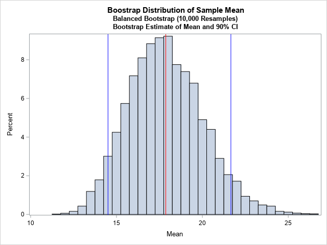
For completeness, the following graph shows the bootstrap distribution for the balanced samples. The red line indicates the bootstrap estimate for the mean, which is the same as the sample mean on the original data. The blue lines represent the 5th and 95th percentiles of the distribution and are therefore estimates for a 90% confidence interval for the population mean.

Should you use the balanced bootstrap?

Should you use the balanced bootstrap method instead of the traditional bootstrap method? In practice, I don't think it matters much which method you use: The inferences that you make should not depend strongly on the method. For example, if you are trying to obtain a confidence interval for a parameter, the estimates should be similar.

On the other hand, there are no major drawbacks to the balanced bootstrap. It provides estimates that are the same as or, on occasion, better than the traditional bootstrap sampling method. So, if it is easy to get a balanced bootstrap sample (as it is in SAS), you might as well use it.

I think the balanced bootstrap is preferred if the data includes an extreme outlier. Look back at the section that used PROC FREQ to examine the frequency that each observation was selected in the traditional bootstrap analysis. You can see that some observations are chosen more than others. These frequencies change if you change the random number seed. Accordingly, some seeds select an outlier more often than other seeds. If you use a seed that selects the outlier many times, the bootstrap distribution will include many extreme statistics. If you change the seed, the new bootstrap distribution might include fewer extreme statistics. The balanced bootstrap removes that uncertainty from your analysis: you know that the outlier appears exactly B times among the set of all B bootstrap samples.

Summary

The METHOD=BALBOOT method in PROC SURVEYSELECT enables you to generate balanced bootstrap resamples. You can analyze these resamples in the same way that you analyze traditional bootstrap resamples. A balanced bootstrap removes one element of uncertainty from your bootstrap estimates. You know that each observation was selected the same number of times over the set of all resamples. This might be comforting if your data contain some extreme outliers, and you want to be certain that the outliers are not overrepresented in the resamples. In this situation, I expect the balanced bootstrap to reduce some of the seed-to-seed variability that you might see in the traditional bootstrap.

Do you have experience with using the balanced bootstrap for real data analysis? Share your experience and thoughts by leaving a comment.