Last week I showed how to use the simple bootstrap to randomly resample from the data to create B bootstrap samples, each containing N observations. The simple bootstrap is equivalent to sampling from the empirical cumulative distribution function (ECDF) of the data. An alternative bootstrap technique is called the smooth bootstrap. In the smooth bootstrap you add a small amount of random noise to each observation that is selected during the resampling process. This is equivalent to sampling from a kernel density estimate, rather than from the empirical density.

The example in this article is adapted from Chapter 15 of Wicklin (2013), Simulating Data with SAS.

The bootstrap method in SAS/IML

My previous article used the bootstrap method to investigate the sampling distribution of the skewness statistic for the SepalWidth variable in the Sashelp.Iris data. I used PROC SURVEYSELECT to resample the data and used PROC MEANS to analyze properties of the bootstrap distribution. You can also use SAS/IML to implement the bootstrap method.

The following SAS/IML statements creates 5000 bootstrap samples of the SepalWidth data. However, instead of computing a bootstrap distribution for the skewness statistic, this program computes a bootstrap distribution for the median statistic. The SAMPLE function enables you to resample from the data.

data sample(keep=x);
   set Sashelp.Iris(where=(Species="Virginica") rename=(SepalWidth=x));
run;
 
/* Basic bootstrap confidence interval for median  */
%let NumSamples = 5000;                 /* number of bootstrap resamples */
proc iml;
use Sample;  read all var {x};  close Sample;        /* read data */
call randseed(12345);                   /* set random number seed */
obsStat = median(x);                    /* compute statistic on original data */
s = sample(x, &NumSamples // nrow(x));  /* bootstrap samples: 50 x NumSamples */
D = T( median(s) );                     /* bootstrap distribution for statistic */
call qntl(q, D, {0.025 0.975});         /* basic 95% bootstrap CI */
results = obsStat || q`;
print results[L="Bootstrap Median" c={"obsStat" "P025" "P975"}];

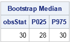
The SAS/IML program is very compact. The MEDIAN function computes the median for the original data. The SAMPLE function generates 5000 resamples; each bootstrap sample is a column of the s matrix. The MEDIAN function then computes the median of each column. The QNTL subroutine computes a 95% confidence interval for the median as [28, 30]. (Incidentally, you can use PROC UNIVARIATE to compute distribution-free confidence intervals for standard percentiles such as the median.)

The bootstrap distribution of the median

The following statement create a histogram of the bootstrap distribution of the median:

title "Bootstrap Distribution for Median";
call histogram(D) label="Median";           /* create histogram in SAS/IML */

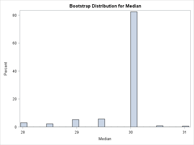
I was surprised when I first saw a bootstrap distribution like this. The distribution contains discrete values. More than 80% of the bootstrap samples have a median value of 30. The remaining samples have values that are integers or half-integers.

This distribution is typical of the bootstrap distribution for a percentile. Three factors contribute to the shape:

• The measurements are rounded to the nearest millimeter. Thus the data are discrete integers.
• The sample median is always a data value or (for N even) the midpoint between two data values. In fact, this statement is true for all percentiles.
• In the Sample data, the value 30 is not only the median, but is the mode. Consequently, many bootstrap samples will have 30 as the median value.

Smooth bootstrap

Although the bootstrap distribution for the median is correct, it is somewhat unsatisfying. Widths and lengths represent continuous quantities. Consequently, the true sampling distribution of the median statistic is continuous.

The bootstrap distribution would look more continuous if the data had been measured with more precision. Although you cannot change the data, you can change the way that you create bootstrap samples. Instead of drawing resamples from the (discrete) ECDF, you can randomly draw samples from a kernel density estimate (KDE) of the data. The resulting samples will not contain data values. Instead, they will contains values that are randomly drawn from a continuous KDE.

You have to make two choices for the KDE: the shape of the kernel and the bandwidth. This article explores two possible choices:

• Uniform kernel: A recorded measurement of 30 mm means that the true value of the sepal was in the interval [29.5, 30.5). In general, a recorded value of x means that the true value is in [x-0.5, x+0.5). Assuming that any point in that interval is equally likely leads to a uniform kernel with bandwidth 0.5.
• Normal kernel: You can assume that the true measurement is normally distributed, centered on the measured value, and is very likely to be within [x-0.5, x+0.5). For a normal distribution, 95% of the probability is contained in ±2σ of the mean, so you could choose σ=0.25 and assume that the true value for the measurement x is in the distribution N(x, 0.25).

For more about the smooth bootstrap, see Davison and Hinkley (1997) Bootstrap Methods and their Application.

Smooth bootstrap in SAS/IML

For the iris data, the uniform kernel seems intuitively appealing. The following SAS/IML program defines a function named SmoothUniform that randomly chooses B samples and adds a random U(-h, h) variate to each data point. The medians of the columns form the bootstrap distribution.

/* randomly draw a point from x. Add noise from U(-h, h) */
start SmoothUniform(x, B, h);
   N = nrow(x) * ncol(x);
   s = Sample(x, N // B);               /* B x N matrix */
   eps = j(B, N);                       /* allocate vector */
   call randgen(eps, "Uniform", -h, h); /* fill vector */
   return( s + eps );                   /* add random uniform noise */
finish;
 
s = SmoothUniform(x, &NumSamples, 0.5); /* columns are bootstrap samples from KDE */
D = T( median(s) );                     /* median of each col is bootstrap distrib */
BSEst = mean(D);                        /* bootstrap estimate of median */
call qntl(q, D, {0.025 0.975});         /* basic 95% bootstrap CI */
results = BSEst || q`;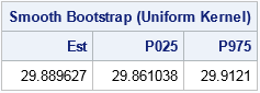
print results[L="Smooth Bootstrap (Uniform Kernel)" c={"Est" "P025" "P975"}];

The smooth bootstrap distribution (not shown) is continuous. The mean of the distribution is the bootstrap estimate for the median. The estimate for this run is 29.8. The central 95% of the smooth bootstrap distribution is [29.77, 29.87]. The bootstrap estimate is close to the observed median, but the CI is much smaller than the earlier simple CI. Notice that the observed median (which is computed on the rounded data) is not in the 95% CI from the smooth bootstrap distribution.

Many researchers in density estimation state that the shape of the kernel function does not have a strong impact on the density estimate (Scott (1992), Multivariate Density Estimation, p. 141). Nevertheless, the following SAS/IML statements define a function called SmoothNormal that implements a smoothed bootstrap with a normal kernel:

/* Smooth bootstrap with normal kernel and sigma = h */
start SmoothNormal(x, B, h);
   N = nrow(x) * ncol(x);
   s = Sample(x, N // B);                /* B x N matrix */
   eps = j(B, N);                        /* allocate vector */
   call randgen(eps, "Normal", 0, h);    /* fill vector */
   return( s + eps );                    /* add random normal variate */
finish;
 
s = SmoothNormal(x, &NumSamples, 0.25);  /* bootstrap samples from KDE */

The mean of this smooth bootstrap distribution is 29.89. The central 95% interval is [29.86, 29.91]. As expected, these values are similar to the values obtained by using the uniform kernel.

Summary of the smooth bootstrap

In summary, the SAS/IML language provides a compact and efficient way to implement the bootstrap method for a univariate statistic such as the skewness or median. A visualization of the bootstrap distribution of the median reveals that the distribution is discrete due to the rounded data values and the statistical properties of percentiles. If you choose, you can "undo" the rounding by implementing the smooth bootstrap method. The smooth bootstrap is equivalent to drawing bootstrap samples from a kernel density estimate of the data. The resulting bootstrap distribution is continuous and gives a smaller confidence interval for the median of the population.