A frequent topic on SAS discussion forums is how to check the assumptions of an ordinary least squares linear regression model. Some posts indicate misconceptions about the assumptions of linear regression. In particular, I see incorrect statements such as the following:

• Help! A histogram of my variables shows that they are not normal! I need to apply a normalizing transformation before I can run a regression....
• Before I run a linear regression, I need to test that my response variable is normal....

Let me be perfectly clear: The variables in a least squares regression model do not have to be normally distributed. I'm not sure where this misconception came from, but perhaps people are (mis)remembering an assumption about the errors in an ordinary least squares (OLS) regression model. If the errors are normally distributed, you can prove theorems about inferential statistics such as confidence intervals and hypothesis tests for the regression coefficients. However, the normality-of-errors assumption is not required for the validity of the parameter estimates in OLS. For the details, the Wikipedia article on ordinary least squares regression lists four required assumptions; the normality of errors is listed as an optional fifth assumption.

In practice, analysts often "check the assumptions" by running the regression and then examining diagnostic plots and statistics. Diagnostic plots help you to determine whether the data reveal any deviations from the assumptions for linear regression. Consequently, this article provides a "getting started" example that demonstrates the following:

1. The variables in a linear regression do not need to be normal for the regression to be valid.
2. You can use the diagnostic plots that are produced automatically by PROC REG in SAS to check whether the data seem to satisfy some of the linear regression assumptions.

By the way, don't feel too bad if you misremember some of the assumptions of linear regression. Williams, Grajales, and Kurkiewicz (2013) point out that even professional statisticians sometimes get confused. And if you want to be pedantic, checking the residuals after a model is run is not proof that the modeling assumptions are true!

An example of nonnormal data in regression

Consider this thought experiment: Take any explanatory variable, X, and define Y = X. A linear regression model perfectly fits the data with zero error. The fit does not depend on the distribution of X or Y, which demonstrates that normality is not a requirement for linear regression.

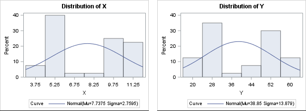
For a numerical example, you can simulate data such that the explanatory variable is binary or is clustered close to two values. The following data shows an X variable that has 20 values near X=5 and 20 values near X=10. The response variable, Y, is approximately five times each X value. (This example is modified from an example in Williams, Grajales, and Kurkiewicz, 2013.) Neither variable is normally distributed, as shown by the output from PROC UNIVARIATE:

/* For n=1..20, X ~ N(5, 1). For n=21..40, X ~ N(10, 1).
   Y = 5*X + e, where e ~ N(0,1) */
data Have;
input X Y @@;
datalines;
 3.60 16.85  4.30 21.30  4.45 23.30  4.50 21.50  4.65 23.20 
 4.90 25.30  4.95 24.95  5.00 25.45  5.05 25.80  5.05 26.05 
 5.10 25.00  5.15 26.45  5.20 26.10  5.40 26.85  5.45 27.90 
 5.70 28.70  5.70 29.35  5.90 28.05  5.90 30.50  6.60 33.05 
 8.30 42.50  9.00 45.50  9.35 46.45  9.50 48.40  9.70 48.30 
 9.90 49.80 10.00 48.60 10.05 50.25 10.10 50.65 10.30 51.20 
10.35 49.80 10.50 53.30 10.55 52.15 10.85 56.10 11.05 55.15 
11.35 55.95 11.35 57.90 11.40 57.25 11.60 57.95 11.75 61.15 
;
 
proc univariate data=Have;
   var x y;
   histogram x y / normal;
run;

There is no need to "normalize" these data prior to performing an OLS regression, although it is always a good idea to create a scatter plot to check whether the variables appear to be linearly related. When you regress Y onto X, you can assess the fit by using the many diagnostic plots and statistics that are available in your statistical software. In SAS, PROC REG automatically produces a diagnostic panel of graphs and a table of fit statistics (such as R-squared):

/* by default, PROC REG creates a FitPlot, ResidualPlot, and a Diagnostics panel */
ods graphics on;
proc reg data=Have;
   model Y = X;
quit;

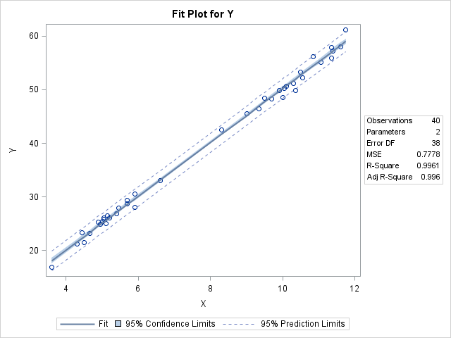
The R-squared value for the model is 0.9961, which is almost a perfect fit, as seen in the fit plot of Y versus X.

Using diagnostic plots to check the assumptions of linear regression

You can use the graphs in the diagnostics panel to investigate whether the data appears to satisfy the assumptions of least squares linear regression. The panel is shown below (click to enlarge).

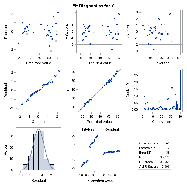
The first column in the panel shows graphs of the residuals for the model. For these data and for this model, the graphs show the following:

• The top-left graph shows a plot of the residuals versus the predicted values. You can use this graph to check several assumptions: whether the model is specified correctly, whether the residual values appear to be independent, and whether the errors have constant variance (homoscedastic). The graph for this model does not show any misspecification, autocorrelation, or heteroscedasticity.
  • A misspecified model would show a systematic trend, such as a quadratic effect that might need to be included in the model.
  • Heteroscedasticity often appears as a "fan-shaped" plot in which the size of the residuals tend to be small on one side of the plot and large on the other.
  • Correlated errors show up as a sequence of consecutive high or low values, rather than a "random scatter" of points.
• The middle-left and bottom-left graphs indicate whether the residuals are normally distributed. The middle plot is a normal quantile-quantile plot. The bottom plot is a histogram of the residuals overlaid with a normal curve. Both these graphs indicate that the residuals are normally distributed. This is evidence that you can trust the p-values for significance and the confidence intervals for the parameters.

In summary, I wrote this article to addresses two points:

1. To dispel the myth that variables in a regression need to be normal. They do not. However, you should check whether the residuals of the model are approximately normal because normality is important for the accuracy of the inferential portions of linear regression such as confidence intervals and hypothesis tests for parameters. (A colleague mentioned to me that standard errors and hypothesis tests tend to be robust to this assumption, so a modest departure from normality is often acceptable.)
2. To show that the SAS regression procedures automatically provide many graphical diagnostic plots that you can use to assess the fit of the model and check some assumptions for least squares regression. In particular, you can use the plots to check the independence of errors, the constant variance of errors, and the normality of errors.

References

There have been many excellent books and papers that describe the various assumptions of linear regression. I don't feel a need to rehash what has already been written, In addition to the Wikipedia article about ordinary linear regression, I recommend the following:

• Frost, J. (2018), "7 Classical Assumptions of Ordinary Least Squares (OLS) Linear Regression," Statistics By Jim blog. Accessed 19Aug2018. This is a nice overview and summary of the assumptions and why they matter.
• Williams, M., Grajales, C., and Kurkiewicz, D. (2013), "Assumptions of Multiple Regression: Correcting Two Misconceptions," Practical Assessment, Research & Evaluation, 18(11). This discusses two common misconceptions and summarizes the assumptions.