As an example, when using ordinary least squares regression (OLS), if your response or dependent attribute’s residuals are not normally distributed, your analysis is likely going to be affected and typically not in a good way. The farther away your input data is from normality, the impact on your model will be as well. One of the assumptions in OLS and is that the residuals of errors of the distribution of the dependent be at least approximately normally distributed³ and this may not affect the parameter estimates but will affect the hypothesis tests such as the p-values derived from the variance and the confidence intervals will be affected as well. A good way to test the residuals is to use a Q-Q plot which can be done using SAS Proc Univariate⁴.

This blog post discusses two distributional data transforms: the natural (or common) logarithm, and the Johnson family of transforms,¹ specifically the Su transform. The Su transform has been empirically shown to improve logistic regression performance from the input attributes.² I will focus primarily on the response or dependent attribute.

Data set example

In this example, the attribute called VALUE24 is the amount of revenue generated from campaign purchases that were obtained in the last 24 months. The histogram below shows the distribution, and the fitted line is what a normal distribution should look like given the mean and variance of this data.

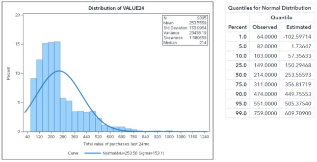
You can clearly see that the normal curve overlaid on the histogram indicates that the data isn’t close to a normal distribution. The dependent attribute of VALUE24 will need to be transformed.

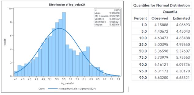
The following histogram is shown with the VALUE24 attributed transform with a natural logarithm. The normal curve is also plotted as before. While this logarithm transform is much better because the normal curve is closer to the log-normal distribution, it still has some room for improvement.

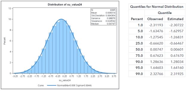
Below is the Su transformed distribution of VALUE24. Notice that not only did it transform it to conform to a normal distribution, it also centered the mean at zero and the variance is one!

Benefits of the Su transform

The benefits of using this transform for use in predictive models are:

• Uses a link-free consistency by allowing an elliptically contoured predictor space.
• Reduction in nonlinear confounding that will lead to less misspecification.
• Local adaptivity: suitable transforms allow models to balance their sensitivity to dense versus sparse regions of the predictor space.²

For details about the first listed benefit, please refer to Potts.² The second benefit is that your model has a much greater chance of being specified correctly due to a reduction in confounding of attributes. This will not only improve your model’s accuracy but its interpretability, as well. The last major benefit is that the Su transform brings in very long tails of a distribution much better than a log or other transforms.¹

Computing the Su transform

The transform that makes the distribution work the best for global smoothing without resorting to a nonparametric density estimation is to estimate a Beta distribution, which can be very close to a normal distribution when certain parameters of the Beta distribution are set.² The actual equation for a Su family is below. However, we won’t be using that exact equation.

What we need is to frame the above equation for the optimal transformation that can be estimated using nonlinear regression and normal scores as the response variable. The above equation can be framed to the following²:

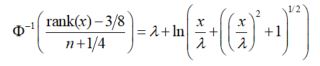
In SAS, one can use the RANK procedure and the nonlinear regression procedure, PROC NLIN; or if using the completely in-memory platform of SAS Viya, PROC NLMOD to accomplish solving the three parameters λ, δ, γ.

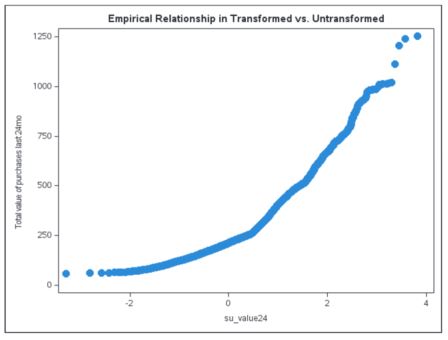
However, there is one serious downside to fitting a Su transform with the above nonlinear function.  Unlike the log or some other transforms, it doesn’t have an inverse link function to transform the data back to its original form. There is one saving grace, however, and that is one can perform an empirical data simulation and develop score code that will mimic the relationship between the Su transformed and the untransformed data. This will enable the Su transform to be estimated on a good statistical representative sample and applied to the larger data set from which the sample was derived. The scatter plot below shows the general relationship of VALUE24 and the Su transformed VALUE24.

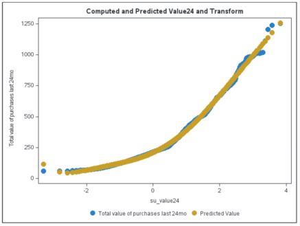
Using PROC GENSELECT, the empirical fit of the above relationship can be performed and score code generated. While other SAS procedures can be used to do the same fitting, such as the TRANSREG and GLMSELECT procedures, they won’t write out the score code at present when using computed effect statements. After fitting this data with a six-degree polynomial spline, the fitted curve is shown in the scatter plot below.

The following SAS score code was generated from the GENSELECT procedure and written to a .sas file on the server.

SAS code used to fit the six-degree curve

ods graphics on;
 
title 'General Smoothing Spline for Value24 Empirical Link Function';
 
proc genselect data=casuser.merge_buytest ;
 
effect poly_su24 = poly( su_value24 /degree=6);
 
model value24 = poly_su24 / distribution=normal;
 
code file="/shared/users/racoll/poly_value24_score.sas";
 
output out=casuser.glms_out pred=pred_value24 copyvar=id;
 
run; title;

Generated SAS scoring code from PROC GENSELECT

drop _badval_ _linp_ _temp_ _i_ _j_; 
_badval_ = 0; _
linp_   = 0; 
_temp_   = 0; 
_i_      = 0; 
_j_      = 0; 
drop MACLOGBIG; 
MACLOGBIG= 7.0978271289338392e+02; 
array _xrow_0_0_{7} _temporary_; 
array _beta_0_0_{7} _temporary_ (    210.154143004534 
    123.296571835751 
    49.7657489425605 
    9.82725091766856 
    -3.13300266038598 
    -0.70029417420551 
    0.17335174313709); 
array _xtmp_0_0_{7} _temporary_; 
array _xcomp_0_0_{7} _temporary_; 
array _xpoly1_0_0_{7} _temporary_;  
 if missing(su_value24) 
 then do; 
    _badval_ = 1; 
    goto skip_0_0; 
end;   
 
do _i_=1 to 7; _xrow_0_0_{_i_} = 0; end; 
do _i_=1 to 7; _xtmp_0_0_{_i_} = 0; end; 
do _i_=1 to 7; _xcomp_0_0_{_i_} = 0; end; 
do _i_=1 to 7; _xpoly1_0_0_{_i_} = 0; end;   
 
_xtmp_0_0_[1] = 1;   
 
_temp_ = 1; 
_xpoly1_0_0_[1] = su_value24; 
_xpoly1_0_0_[2] = su_value24 * _xpoly1_0_0_[1];
 _xpoly1_0_0_[3] = su_value24 * _xpoly1_0_0_[2]; 
_xpoly1_0_0_[4] = su_value24 * _xpoly1_0_0_[3]; 
_xpoly1_0_0_[5] = su_value24 * _xpoly1_0_0_[4];
 _xpoly1_0_0_[6] = su_value24 * _xpoly1_0_0_[5]; 
do _j_=1 to 1; _xtmp_0_0_{1+_j_} = _xpoly1_0_0_{_j_}; end;   
 
_temp_ = 1; 
do _j_=1 to 1; _xtmp_0_0_{2+_j_} = _xpoly1_0_0_{_j_+1}; end; 
_temp_ = 1; 
do _j_=1 to 1; _xtmp_0_0_{3+_j_} = _xpoly1_0_0_{_j_+2}; end; 
_temp_ = 1; 
do _j_=1 to 1; _xtmp_0_0_{4+_j_} = _xpoly1_0_0_{_j_+3}; end; 
_temp_ = 1; 
do _j_=1 to 1; _xtmp_0_0_{5+_j_} = _xpoly1_0_0_{_j_+4}; end; 
_temp_ = 1; 
do _j_=1 to 1; _xtmp_0_0_{6+_j_} = _xpoly1_0_0_{_j_+5}; end; 
do _j_=1 to 1; _xrow_0_0_{_j_+0} = _xtmp_0_0_{_j_+0}; end; 
do _j_=1 to 1; _xrow_0_0_{_j_+1} = _xtmp_0_0_{_j_+1}; end; 
do _j_=1 to 1; _xrow_0_0_{_j_+2} = _xtmp_0_0_{_j_+2}; end; 
do _j_=1 to 1; _xrow_0_0_{_j_+3} = _xtmp_0_0_{_j_+3}; end; 
do _j_=1 to 1; _xrow_0_0_{_j_+4} = _xtmp_0_0_{_j_+4}; end; 
do _j_=1 to 1; _xrow_0_0_{_j_+5} = _xtmp_0_0_{_j_+5}; end; 
do _j_=1 to 1; _xrow_0_0_{_j_+6} = _xtmp_0_0_{_j_+6}; end;  
 
do _i_=1 to 7; 
_linp_ + _xrow_0_0_{_i_} * _beta_0_0_{_i_}; 
end;   
 
skip_0_0: 
label P_VALUE24 = 'Predicted: VALUE24'; 
if (_badval_ eq 0) and not missing(_linp_) then do; 
  P_VALUE24 = _linp_; 
end; else do; 
    _linp_ = .; 
    P_VALUE24 = .; 
end;

This score code can be placed in a SAS DATA step along with your analytical model’s score code so that a back-transform can be accomplished of your predicted dependent variable VALUE24.

If you liked this blog post, then you might like my latest book, Segmentation Analytics with SAS® Viya®: An Approach to Clustering and Visualization.

References

¹ Johnson, N. L., “Systems of Frequency Curves Generated by Methods of Translation,” Biometrika, 1949.

² Potts, W., “Elliptical Predictors for Logistic Regression”, Keynote Address at SAS Data Mining Conference, Las Vegas, NV, 2006.

³ Wikipedia article on OLS regression: https://en.wikipedia.org/wiki/Ordinary_least_squares#Classical_linear_regression_model

⁴ Wicklin, R. “On the assumptions (and misconceptions) of linear regression, SAS Blog article, 2018. On the assumptions (and misconceptions) of linear regression - The DO Loop (sas.com)