Bootstrap regression estimates: Residual resampling

If you want to bootstrap the parameters in a statistical regression model, you have two primary choices. The first, case resampling, is discussed in a previous article. This article describes the second choice, which is resampling residuals (also called model-based resampling). This article shows how to implement residual resampling in Base SAS and in the SAS/IML matrix language.

Residual resampling assumes that the model is correctly specified and that the error terms in the model are identically distributed and independent. However, the errors do not need to be normally distributed. Before you run a residual-resampling bootstrap, you should use regression diagnostic plots to check whether there is an indication of heteroskedasticity or autocorrelation in the residuals. If so, do not use this bootstrap method.

Although residual resampling is primarily used for designed experiments, this article uses the same data set as in the previous article: the weights (Y) and heights (X) of 19 students. Therefore, you can compare the results of the two bootstrap methods. As in the previous article, this article uses the bootstrap to examine the sampling distribution and variance of the parameter estimates (the regression coefficients).

Bootstrap residuals

The following steps show how to bootstrap residuals in a regression analysis:

Fit a regression model that regresses the original response, Y, onto the explanatory variables, X. Save the predicted values (Y_Pred) and the residual values (R).
A bootstrap sample consists of forming a new response vector as Y_{i, Boot} = Y_{i, Pred} + R_rand, where Y_{i, Pred} is the i_th predicted value and R_rand is chosen randomly (with replacement) from the residuals in Step 1. Create B samples, where B is a large number.
For each bootstrap sample, fit a regression model that regresses Y_Boot onto X.
The bootstrap distribution is the union of all the statistics that you computed in Step 3. Analyze the bootstrap distribution to estimate standard errors and confidence intervals for the parameters.

Step 1: Fit a model, save predicted and residual values

To demonstrate residual resampling, I will use procedures in Base SAS and SAS/STAT. (A SAS/IML solution is presented at the end of this article.) The following statements create the data and rename the response variable (Weight) and the explanatory variable (X) so that their roles are clear. Step 1 of the residual bootstrap is to fit a model and save the predicted and residual values:

data sample(keep=x y);
   set Sashelp.Class(rename=(Weight=Y Height=X));
run;
 
/* 1. compute value of the statistic on original data */
proc reg data=Sample plots=none;
   model Y = X / CLB covb;
   output out=RegOut predicted=Pred residual=Resid;
run; quit;
 
%let IntEst = -143.02692;  /* set some macro variables for later use */
%let XEst   =    3.89903;
%let nObs   =   19;

Step 2: Form the bootstrap resamples

The second step is to randomly draw residuals and use them to generate new response vectors from the predicted values of the fitted model. There are several ways to do this. If you have SAS 9.4m5 (SAS/STAT 14.3), you can use PROC SURVEYSELECT to select and output the residuals in a random order. An alternative method that uses the SAS DATA step is shown below. The program reads the residuals into an array. For each original observation, it adds a random residual to the predicted response. It does this B times, where B = 5,000. It then sorts the data by the SampleID variable so that the B bootstrap samples are ready to be analyzed.

%let NumSamples = 5000;             /* B = number of bootstrap resamples */
/* SAS macro: chooses random integer in [min, max]. See
   https://blogs.sas.com/content/iml/2015/10/05/random-integers-sas.html */
%macro RandBetween(min, max);
   (&min + floor((1+&max-&min)*rand("uniform")))
%mend;
 
/* 2. For each obs, add random residual to predicted values to create 
      a random response. Do this B times to create all bootstrap samples. */
data BootResiduals;
array _residual[&nObs] _temporary_; /* array to hold residuals */
do i=1 to &nObs;                    /* read data; put rasiduals in array */
   set RegOut point=i;
   _residual[i] = Resid;
end;
 
call streaminit(12345);             /* set random number seed */
set RegOut;                         /* for each observations in data */
ObsID = _N_;                        /* optional: keep track of obs position */
do SampleId = 1 to &NumSamples;     /* for each bootstrap sample */
   k = %RandBetween(1, &nObs);      /* choose a random residual */
   YBoot = Pred + _residual[k];     /* add it to predicted value to create new response */
   output;
end;
drop k;
run;
 
/* prepare for BY group analysis: sort by SampleID */
proc sort data=BootResiduals;
by SampleID ObsID;                  /* sorting by ObsID is optional */
run;

Step 3: Analyze the bootstrap resamples

The previous step created a SAS data set (BootResiduals) that contains B = 5,000 bootstrap samples. The unique values of the SampleID variable indicate which observations belong to which sample. You can use a BY-group analysis to efficiently analyze all samples in a single call to PROC REG, as follows:

/* 3. analyze all bootstrap samples; save param estimates in data set  */
proc reg data=BootResiduals noprint outest=PEBootResid; 
   by SampleID;
   model YBoot = X;
run;quit;
 
/* take a peek at the first few bootstrap estimates */
proc print data=PEBootResid(obs=5);
   var SampleID Intercept X;
run;

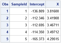
The result of the analysis is a data set (PEBootResid) that contains 5,000 rows. The i_th row contains the parameter estimates for the i_th bootstrap sample. Thus, the Intercept and X columns contain the bootstrap distribution of the parameter estimates, which approximates the sampling distribution of those statistics.

Step 4: Analyze the bootstrap distribution

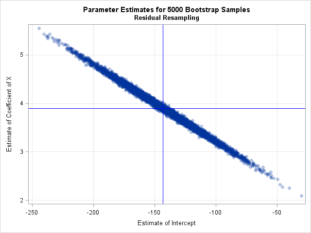
The previous article includes SAS code that estimates the standard errors and covariance of the parameter estimates. It also provides SAS code for a bootstrap confidence interval for the parameters. I will not repeat those computations here. The following call to PROC SGPLOT displays a scatter plot of the bootstrap distribution of the estimates. You can see from the plot that the estimates are negatively correlated:

/* 4. Visualize and analyze the bootstrap distribution */
title "Parameter Estimates for &NumSamples Bootstrap Samples";
title2 "Residual Resampling";
proc sgplot data=PEBootResid;
   label Intercept = "Estimate of Intercept" X = "Estimate of Coefficient of X";
   scatter x=Intercept y=X / markerattrs=(Symbol=CircleFilled) transparency=0.7;
   /* Optional: draw reference lines at estimates for original data */
   refline &IntEst / axis=x lineattrs=(color=blue);
   refline &XEst / axis=y lineattrs=(color=blue);
   xaxis grid; yaxis grid;
run;

Bootstrap residuals in SAS/IML

For standard regression analyses, the previous sections show how to bootstrap residuals in a regression analysis in SAS. If you are doing a nonstandard analysis, however, you might need to perform a bootstrap analysis in the SAS/IML language. I've previously shown how to perform a bootstrap analysis (using case resampling) in SAS/IML. I've also shown how to use the SWEEP operator in SAS/IML to run thousands of regressions in a single statement. You can combine these ideas, along with an easy way to resample data (with replacement) in SAS/IML, to write a short SAS/IML program that resamples residuals, fits the samples, and plots the bootstrap estimates:

proc iml;
use RegOut;  read all var {Pred X Resid};  close; /* read data */
design = j(nrow(X), 1, 1) || X;           /* design matrix for explanatory variables */
 
/* resample residuals with replacement; form bootstrap responses */
call randseed(12345);
R = sample(Resid, &NumSamples//nrow(Resid)); /* NxB matrix; each col is random residual */
YBoot = Pred + R;                         /* 2. NxB matrix; each col is Y_pred + resid */
M = design || YBoot;                      /*    add intercept and X columns */
ncol = ncol(M);
MpM = M`*M;                               /*    (B+2) x (B+2) crossproduct matrix */
free R YBoot M;                           /*    free memory */
 
/* Use SWEEP function to run thousands of regressions in a single call */
S = sweep(MpM, {1 2});                    /* 3. sweep in intercept and X for each Y_i */
ParamEst = S[{1 2}, 3:ncol];              /*    estimates for models Y_i = X */
 
/* 4. perform bootstrap analyses by analyzing ParamEst */
call scatter(ParamEst[1,], ParamEst[2,]) grid={x y} label={"Intercept" "X"}
     other="refline &IntEst /axis=x; refline &XEst /axis=y;";

The graph is similar to the previous scatter plot and is not shown. It is remarkable how concise the SAS/IML language can be, especially compared to the procedure-based approach in Base SAS. On the other hand, the SAS/IML program uses a crossproduct matrix (MpM) that contains approximately B² elements. If you want to analyze, say, B = 100,000 bootstrap samples, you would need to restructure the program. For example, you could analyze 10,000 samples at a time and accumulate the bootstrap estimates.

Further thoughts and summary

The %BOOT macro also supports resampling residuals in a regression context. The documentation for the %BOOT macro contains an example. No matter how you choose to bootstrap residuals, remember that the process assumes that the model is correct and that the error terms in the model are identically distributed and independent.

Use caution if the response variable has a physical meaning, such as a physical dimension that must be positive (length, weight, ...). When you create a new response as the sum of a predicted value and a random residual, you might obtain an unrealistic result, especially if the data contain an extreme outlier. If your resamples contain a negative length or a child whose height is two meters, you might reconsider whether resampling residuals is appropriate for your data and model.

When it is appropriate, the process of resampling residuals offers a way to use the bootstrap to investigate the variance of many parameters that arise in regression. It is especially useful for data from experiments in which the explanatory variables have values that are fixed by the design.

Blogs