SAS programmers on SAS discussion forums sometimes ask how to run thousands of regressions of the form Y = B0 + B1*X_i, where i=1,2,.... A similar question asks how to solve thousands of regressions of the form Y_i = B0 + B1*X for thousands of response variables. I have previously written about how to solve the first problem by converting the data from wide form to a long form and using the BY statement in PROC REG to solve the thousands of regression problems in a single call to the procedure. My recent description of the SWEEP operator (which is implemented in SAS/IML software), provides an alternative technique that enables you to analyze both regression problems when the data are in the wide format.

Why would you anyone need to run 1,000 regressions?

Why anyone wants to solve thousands of linear regression problems? I can think of a few reasons:

1. In the exploratory phase of an analysis, you might want to know which of thousands of variables are linearly related to a response. Running the regressions is a quick way to filter or "screen out" variables that do not have a strong linear association with the response.
2. In a simulation study, each Y_i might be an independent draw from the same distribution. Running thousands of regressions enables you to approximate the sampling distribution of the parameter estimates.
3. In a bootstrap analysis of regression estimates, you can perform case resampling or model-based resampling. In case resampling, you generate many X_i by resampling from the original X variable. In model-based resampling, you keep the X fixed and resample thousands of Y_i. In either case, Running thousands of regressions enables you to estimate the precision of the parameter estimates.

Many univariate regressions

In a previous article, I showed how to simulate data that satisfies a regression model. I created a data set that contains explanatory variables X1-X1000 and a single response variable, Y. You can download the SAS program that computes the data and performs the regression.

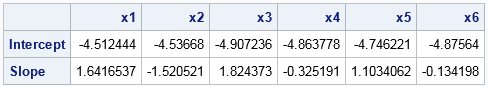
The following SAS/IML program reads the simulated data into a large matrix, M. For each regression, it forms the three-column matrix A from the intercept column, the k_th explanatory variable, and the variable Y. It then forms the sum of squares and cross products (SSCP) matrix (A`*A) and uses the SWEEP function to solve the least squares regression problem. The two parameter estimates (intercept and slope) for each explanatory variable are saved in a 2 x 1000 array. A few parameter estimates are displayed.

/* program to compute parameter estimates for Y = b0 + b1*X_k, k=1,2,... */
proc iml;
XVarNames = "x1":"x&nCont";      /* names of explanatory variables */
p = ncol(XVarNames );            /* number of X variables, excluding intercept */
varNames = XVarNames || "Y";     /* name of all data variables */
use Wide;  read all var varNames into M;  close; /* read data into M */
 
A = j(nrow(M), 3, 1);            /* columns for intercept, X_k, Y */
A[ ,3] = M[ , ncol(M)];          /* put Y in 3rd col */
ParamEst =  j(2, p, .);          /* allocate 2 x p matrix for estimates */
do k = 1 to ncol(XVarNames);
   A[ ,2] = M[ ,k];              /* X_k in 2nd col */
   S1 = sweep(A`*A, {1 2});      /* sweep in intercept and X_k */
   ParamEst[ ,k] = S1[{1 2}, 3]; /* estimates for k_th model Y = b0 + b1*X_k */
end;
print (paramEst[,1:6])[r={"Intercept" "Slope"} c=XVarNames];

You could perform a similar loop for models that contain multiple variables, such as all two-variable main-effect models of the form Y = b0 + b1*X_k + b2*X_j, where k ≠ j. You can use the ALLCOMB function in SAS/IML to choose the combinations of columns to sweep.

One large multivariate regression

You can also use the SWEEP operator to perform the regression of many responses onto a single explanatory variable. This case is easy in PROC REG because the procedure supports multiple response variables. The analysis is also easy if you use the SWEEP function in SAS/IML. It only requires a single function call!

The following DATA step simulates 1,000 response variables according to the model Y_i = b0 + b1*X + ε, where b0 = 39.07, b1 = 0.902, and ε ~ N(0, 5.71) is a normally distributed random error term. These values are the parameter estimates for the regression of SepalLength onto SepalWidth for the virginica species of iris flowers in the Sashelp.Iris data set. For more about simulating regression models, see Chapter 11 of Wicklin (2013).

/* based on Wicklin (2013, p. 203) */
%let NumSim = 1000;                  /* number of Y variables */
data RegSim(drop=RMSE b0 b1 k Species);
set Sashelp.Iris(where =(Species="Virginica") keep=Species SepalWidth
                 rename=(SepalWidth=X));
RMSE = 5.71; b0 = 39.07; b1 = 0.902; /* param estimates for model SepalLength = SepalWidth */
array Y[&NumSim];
call streaminit(321);
do k = 1 to &NumSim;
   Y[k] = b0 + b1*X + rand("Normal", 0, RMSE); /* simulate responses from model */
end;
output;
run;

After generating the data, you can compute all 1,000 parameter estimates by using a single call to the SWEEP function in SAS/IML. The following program forms a matrix M for which the first column is an intercept term, the second column is the X variable, and the next 1,000 columns are the simulated responses. Sweeping the first two rows of the M`*M matrix computes the 1,000 parameter estimates, which are then graphed in a scatter plot.

/* program to compute parameter estimates for Y_k = b0 + b1*X, k=1,2,... */
proc iml;
YVarNames = "Y1":"Y&numSim";     /* names of explanatory variables */
varNames = "X" || YVarNames;     /* name of all data variables */
use RegSim;  read all var varNames into M;  close;
M = j(nrow(M), 1, 1) || M;       /* add intercept column */
 
S1 = sweep(M`*M, {1 2});         /* sweep in intercept and X */
ParamEst = S1[{1 2}, 3:ncol(M)]; /* estimates for models Y_i = X */
 
title "Parameter Estimates for 1,000 Simulated Responses";
call scatter(ParamEst[1,], ParamEst[2,]) label={"Intercept" "X"}
     other="refline 39.07/axis=x; refline 0.902/axis=y;";

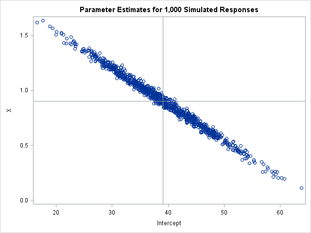
The graph shows the parameter estimates for each of the 1,000 linear regressions. The distribution of the estimates provides more information about the sampling distribution than the estimate of standard error that PROC REG produces when you run a regression model. The graph visually demonstrates the "covariance of the estimates," which PROC REG estimates if you use the COVB option on the MODEL statement.

In summary, you can use the SWEEP operator (implemented in the SWEEP function in SAS/IML) to efficiently compute thousands of regression estimates for wide data. This article demonstrates how to compute models that have many explanatory variables (Y = b0 + b1* X_i) and models that have many response variables (Y_i = b0 + b1 * X). Are there drawbacks to this approach? Sure. You don't automatically get the dozens of ancillary regression statistics like R squared, adjusted R squared, p-values, and so forth. Also, PROC REG automatically handles missing values, whereas in SAS/IML you must first extract the complete cases before you try to form the SSCP matrix. Nevertheless, this computation can be useful for simulation studies in which the data are simulated and analyzed within SAS/IML.

Download the SAS programs for this article.