For ordinary least squares (OLS) regression, you can use a basic bootstrap of the residuals (called residual resampling) to perform a bootstrap analysis of the parameter estimates. This is possible because an assumption of OLS regression is that the residuals are independent. Therefore, you can reshuffle the residuals to get each bootstrap sample.

For a time series, the residuals are not independent. Rather, if you fit a model to the data, the residuals at time t+i are often close to the residual at time t for small values of i. This is known as autocorrelation in the error component. Accordingly, if you want to bootstrap the residuals of a time series, it is not correct to randomly shuffle the residuals, which would destroy the autocorrelation. Instead, you need to randomly choose a block of residuals (for example, at times t, t+1, ..., and t+L) and use those blocks of residuals to create bootstrap resamples. You repeatedly choose random blocks until you have enough residuals to create a bootstrap resample.

There are several ways to choose blocks:

• The simplest way is to choose from non-overlapping blocks of a fixed length, L. This is called the simple block bootstrap and is described in this article.
• Only slightly more complicated is to allow the blocks of length L to overlap. This is called the moving block bootstrap and is described in a second article.
• A more complicated scheme (but which has superior statistical properties) is to allow the length of the blocks to vary. This is called the stationary block bootstrap and is described in a third article.

Create the residuals

There are many ways to fit a model to a time series and to obtain the model residuals. Trovero and Leonard (2018) discuss several modern methods to fit trends, cycles, and seasonality by using SAS 9.4 or SAS Viya. To get the residuals, you will want to fit an additive model. In this article, I will use the Sashelp.Air data and will fit a simple additive model (trend plus noise) by using the AUTOREG procedure in SAS/ETS software.

The Sashelp.Air data set has 144 months of data. The following SAS DATA step drops the first year of data, which leaves 11 years of 12 months. I am doing this because I am going to use blocks of size L=12, and I think the example will be clearer if there are 11 blocks of size 12 (rather than 12 blocks).

data Air;
set Sashelp.Air;
if Date >= '01JAN1950'd;   /* exclude first year of data */
Time = _N_;                /* the observation number */
run;
 
title "Original Series: Air Travel";
proc sgplot data=Air;
   series x=Time y=Air;
   xaxis grid; yaxis grid;
run;

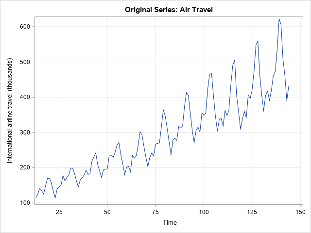
The graph suggests that the time series has a linear trend. The following call to PROC AUTOREG fits a linear model to the data. The predicted mean and residuals are output to the OutReg data set as the PRED and RESID variables, respectively. The call to PROC SGPLOT overlays a graph of the trend and a graph of the residuals.

/* Similar to Getting Started example in PROC AUTOREG */
proc autoreg data=Air plots=none outest=RegEst;
   AR12: model Air = Time / nlag=12;
   output out=OutReg pm=Pred rm=Resid;  /* mean prediction and residuals */
   ods select FinalModel.ParameterEstimates ARParameterEstimates;
run;
 
title "Mean Prediction and Residuals from AR Model";
proc sgplot data=OutReg;
   series x=Time y=Pred;
   series x=Time y=Resid;
   refline 0 / axis=y;
   xaxis values=(24 to 144 by 12) grid valueshint;
run;

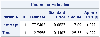
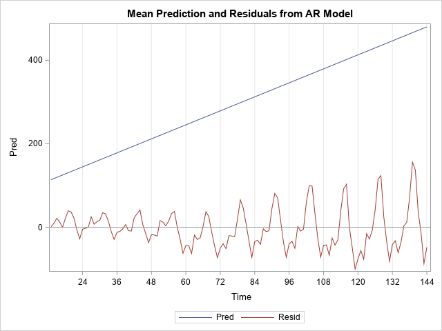
The parameter estimates are shown for the linear model. On average, airlines carried an additional 2.8 thousand passengers per month during this time period. The graph shows the decomposition of the series into a linear trend and residuals. I added vertical lines to indicate the blocks of residuals that are used in the next section. The first block contains the residuals for times 13-24. The second block contains the residuals for times 25-36, and so forth until the 11th block, which contains the residuals for times 133-144.

Set up the simple block bootstrap

For the simple bootstrap, the length of the blocks (L) must evenly divide the length of the series (n), which means that k = n / L is an integer. Because I dropped the first year of observations from Sashelp.Air, there are n=132 observations. I will choose the block size to be L=12, which means that there are k=11 non-overlapping blocks.

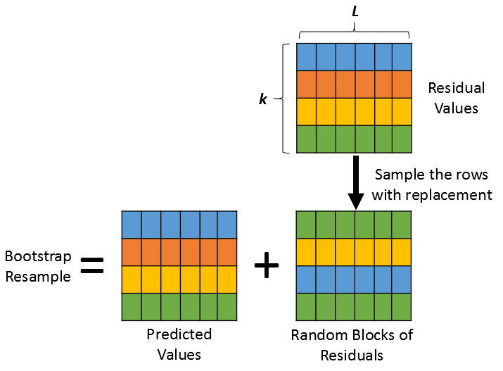
Each bootstrap resample is formed by randomly choosing k blocks (with replacement) and add those residuals to the predicted values. Think about putting the n predicted values and residuals into a matrix in row-wise order. The first L observations are in the first row, the next L are in the second row, and so forth. Thus, the matrix has k rows and L columns. The original series is of the form Predicted + Residuals, where the plus sign represents matrix addition. For the simple block bootstrap, each bootstrap resample is obtained by resampling the rows of the residual array and adding the rows together to obtain a new series of the form Predicted + (Random Residuals). This process is shown schematically in the following figure.

You can use the SAS/IML language to implement the simple block bootstrap. The following call to PROC IML reads in the original predicted and residual values and reshapes then vectors into k x L matrices (P and R, respectively). The SAMPLE function generates a sample (with replacement) of the vector 1:k, which is used to randomly select rows of the R matrix. To make sure that the process is working as expected, you can create one bootstrap resample and graph it. It should resemble the original series:

/* SIMPLE BLOCK BOOTSTRAP */
%let L = 12;
proc iml;
call randseed(12345);
/* the original series is Y = Pred + Resid */
use OutReg;
   read all var {'Time' 'Pred' 'Resid'};
close;
 
/* For the Simple Block Bootstrap, the length of the series (n) 
   must be divisible by the block length (L). */
n = nrow(Pred);          /* length of series */
L = &L;                  /* length of each block */
k = n / L;               /* number of non-overlapping blocks */
if k ^= int(k) then 
   ABORT "The series length is not divisible by the block length";
 
/* Trick: reshape data into k x L matrix. Each row is block of length L */
P = shape(Pred, k, L);
R = shape(Resid, k, L); /* non-overlapping residuals (also k x L) */
 
/* Example: Generate one bootstrap resample by randomly selecting from the residual blocks */
idx = sample(1:nrow(R), k);     /* sample (w/ replacement) of size k from the set 1:k */
YBoot = P + R[idx,];
title "One Bootstrap Resample";
title2 "Simple Block Bootstrap";
refs = "refline " + char(do(12,nrow(Pred),12)) + " / axis=x;";
call series(Time, YBoot) other=refs;

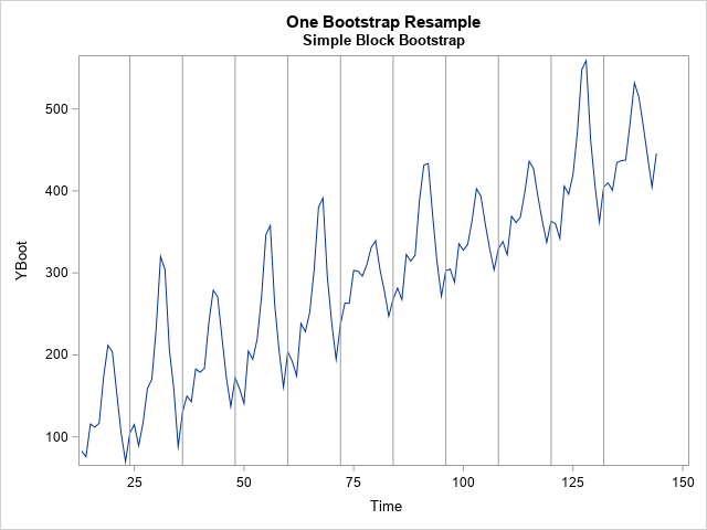
The graph shows one bootstrap resample. The residuals from arbitrary blocks are concatenated until there are n residuals. These are added to the predicted value to create a "new" series, which is a bootstrap resample. You can generate a large number of bootstrap resamples and use them to perform inferences for time series statistics.

Implement the simple block bootstrap in SAS

You can repeat the process in a loop to generate more resamples. The following statements generate B=1000 bootstrap resamples. These are written to a SAS data set (BootOut). The program uses a technique in which the results of each computation are immediately written to a SAS data set, which is very efficient. The program writes the Time variable, the resampled series (YBoot), and an ID variable that identifies each bootstrap sample.

/* The simple block bootstrap repeats this process B times
   and usually writes the resamples to a SAS data set. */
B = 1000;
J = nrow(R);              /* J=k for non-overlapping blocks, but prepare for moving blocks */
SampleID = j(n,1,.);
create BootOut var {'SampleID' 'Time' 'YBoot'};  /* open data set outside of loop */
do i = 1 to B;
   SampleId[,] = i;       /* fill array: https://blogs.sas.com/content/iml/2013/02/18/empty-subscript.html */
   idx = sample(1:J, k);  /* sample of size k from the set 1:k */
   YBoot = P + R[idx,];
   append;                /* append each bootstrap sample */
end;
close BootOut;
QUIT;

The BootOut data set contains B=1000 bootstrap samples. You can efficiently analyze the samples by using a BY statement. For example, suppose that you want to investigate how the parameter estimates for the trend line vary among the bootstrap samples. You can run PROC AUTOREG on each bootstrap sample by using BY-group processing. Be sure to suppress ODS output during the BY-group analysis, and write the desired statistics to an output data set (BootEst), as follows:

/* Analyze the bootstrap samples by using a BY statement. See
   https://blogs.sas.com/content/iml/2012/07/18/simulation-in-sas-the-slow-way-or-the-by-way.html
*/
proc autoreg data=BootOut plots=none outest=BootEst noprint;
   by SampleID;
   AR12: model YBoot = Time / nlag=12;
run;
 
/* OPTIONAL: Use PROC MEANS or PROC UNIVARIATE to estimate standard errors and CIs */
proc means data=BootEst mean stddev P5 P95;
   var Intercept Time _A:;
run;
 
title "Distribution of Parameter Estimates";
proc sgplot data=BootEst;
   scatter x=Intercept y=Time;
   xaxis grid; yaxis grid; 
   refline 77.5402 / axis=x;
   refline 2.7956  / axis=y;
run;

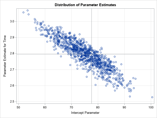
The scatter plot shows the bootstrap distribution of the parameter estimates of the linear trend. The reference lines indicate the parameter estimates for the original data. You can use the bootstrap distribution for inferential statistics such as estimation of standard errors, confidence intervals, the covariance of estimates, and more.

You can perform a similar bootstrap analysis for any other statistic that is generated by any time series analysis. The important thing is that the block bootstrap is performed on some sort of residual or "noise" component, so be sure to remove the trend, seasonality, cycles, and so forth and then bootstrap the remainder.

Summary

This article shows how to perform a simple block bootstrap on a time series in SAS. First, you need to decompose the series into additive components: Y = Predicted + Residuals. You then choose a block length (L), which (for the simple block bootstrap) must divide the total length of the series (n). Each bootstrap resample is generated by randomly choosing blocks of residuals and adding them to the predicted model. This article uses the SAS/IML language to perform the simple block bootstrap in SAS.

In practice, the simple block bootstrap is rarely used. However, it illustrates the basic ideas for bootstrapping a time series, and it provides a foundation for more sophisticated bootstrap methods.