This is the third and last introductory article about how to bootstrap time series in SAS. In the first article, I presented the simple block bootstrap and discussed why bootstrapping a time series is more complicated than for regression models that assume independent errors. Briefly, when you perform residual resampling on a time series, you need to resample in blocks to simulate the autocorrelation in the original series. In the second article, I introduced the moving-block bootstrap. For both methods, all blocks are the same size, and the block size must evenly divide the length of the series (n).

In contrast, the stationary block bootstrap uses blocks of random lengths. This article describes the stationary block bootstrap and shows how to implement it in SAS.

The "stationary" bootstrap gets its name from Politis and Romano (1992), who developed it. When applied to stationary data, the resampled pseudo-time series is also stationary.

Choosing the length of a block

In the moving-block bootstrap, the starting location for a block is chosen randomly, but all blocks have the same length. For the stationary block bootstrap, both the starting location and the length of the block are chosen at random.

The distribution for the block length is typically chosen from a geometric distribution with parameter p. If you want the average block length to be L, define p = 1/L because the expected value of a geometric distribution with parameter p is 1/p.

Why do we choose lengths from the geometric distribution? Well, because a length from the geometric distribution is easy to interpret in terms of a discrete process. Imagine performing the following process:

• Choose an initial location, t, at random.
• With probability p, choose a different location (at random) for the next residual and start a new block.
• With probability (1-p), choose the location t+1 for the next residual and add that residual to the current block.

Generate a random block

There are several ways to implement the stationary block bootstrap in SAS. A straightforward method is to generate a starting integer, t, uniformly at random in the range [1, n], where n is the length of the series. Then, choose a length, L ~ Geom(p). If t + L exceeds n, truncate the block. (Some practitioners "wrap" the block to include residuals at the beginning of the series. This alternative method is called the circular block bootstrap.) Continue this process until the total length of the blocks is n. You will usually need to truncate the length of the last block so that the sum of the lengths is exactly n. This process is implemented in the following SAS/IML user-defined functions:

/* STATIONARY BLOCK BOOTSTRAP */
/* Use a random starting point, t, and a random block length, L ~ Geom(p), 
   - probability p of starting a new block at a new position
   - probability (1-p) of using the next residual from the current block
*/
%let p = (1/12);                /* expected block length is 1/p */ 
proc iml;
/* generate indices for a block of random length L~Geom(p)
   chosen from the sequence 1:n */
start RandBlockIdx(n, p);
   beginIdx = randfun(1, "Integer", n); /* random start: 1:n */
   L = randfun(1, "Geom", p);           /* random length */
   endIdx = min(beginIdx+L-1, n);       /* truncate into 1:n */
   return( beginIdx:endIdx );           /* return sequence of indices in i:n */
finish;
 
/* generate indices for one stationary bootstrap resample */
start StationaryIdx(n, p);
   bootIdx = j(n,1,.);
   s = 1;                       /* starting index for first block */
   do while( s <= n );
      idx = RandBlockIdx(n, p); /* get block of random length */
      if ncol(idx) > n-s then   /* truncate if block too long */
         idx = idx[, 1:n-s+1];
      L = ncol(idx);            /* length of this block */
      jdx = s:s+L-1;            /* all indices for this block */
      bootIdx[jdx] = idx;       /* assign this block */
      s = s + L;                /* starting index for next block */
   end;
   return bootIdx;
finish;

Let's run these functions on some sample data. The first article in this series shows how to fit a model to the Sashelp.Air data and write the predicted and residual values. The following statements use the stationary block bootstrap to generate one bootstrap sample of length n from the residuals. When you add the bootstrapped residuals to the predicted values, you get a "new" time series, which is graphed:

use OutReg;                     /* data to bootstrap: Y = Pred + Resid */
   read all var {'Time' 'Pred' 'Resid'};
close;
 
call randseed(1234);
n = nrow(Pred);                 /* length of series */
prob = &p;                      /* probability of jumping to a new block */
 
/*---- Visualization Example: generate one bootstrap resample ----*/
idx = StationaryIdx(n, prob);
YBoot = Pred + Resid[idx];
 
/* visualize the places where a sequence is not ascending:
https://blogs.sas.com/content/iml/2013/08/28/finite-diff-estimate-maxi.html */
blocksIdx = loc(dif(idx) <= 0); /* where is the sequence not ascending? */
b = Time[blocksIdx];
 
title "One Bootstrap Resample";
title2 "Stationary Block Bootstrap";
refs = "refline " + char(b) + " / axis=x;";
call series(Time, YBoot) other=refs;
/*---- End of visualization example ----*/

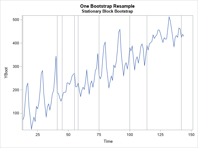
The graph shows a single bootstrap sample. I have added vertical reference lines to show the blocks of residuals. For this random sample, there are nine blocks whose lengths vary between 2 (the last block) and 28. If you choose another random sample, you will get a different set of blocks that have different lengths.

The stationary block bootstrap

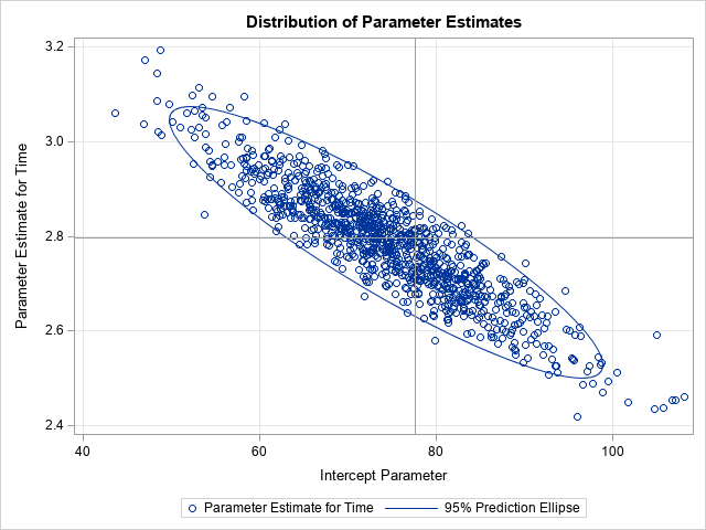
In practice, the bootstrap method requires many bootstrap resamples. You can call the StationaryIdx function repeatedly in a loop to generate B=1000 bootstrap samples, as follows:

/* A complete stationary block bootstrap generates B resamples
   and usually writes the resamples to a SAS data set. */
B = 1000;
SampleID = j(n,1,.);
create BootOut var {'SampleID' 'Time' 'YBoot'};  /* create outside of loop */
do i = 1 to B;
   SampleId[,] = i;   /* fill array. See https://blogs.sas.com/content/iml/2013/02/18/empty-subscript.html */
   idx = StationaryIdx(n, prob);
   YBoot = Pred + Resid[idx];
   append;
end;
close BootOut;

The BootOut data set contains all the bootstrap samples. You can use a BY-group analysis to obtain the bootstrap estimates for almost any statistic. For example, the following scatter plot shows the distribution of 1000 bootstrap estimates of the slope and intercept parameters for an autoregressive model of the series. Reference lines indicate the estimates for the original data.

You can download the complete SAS program that performs all computations and creates all graphs in this article.

Summary

This article is the third of a series. It shows how to perform a stationary block bootstrap by randomly sampling blocks of residuals. Whereas the simple-block and the moving-block bootstrap methods use blocks that have a constant length, the stationary block bootstrap chooses blocks of random lengths.

In researching these blog posts, I read several articles. I recommend Bates (2019) for an introduction and Politis and Romano (1994) for details.

• Bates, Andrew (2019), "Time Series Bootstrap Methods," accessed 17Jan2021.
• Politis, D. N. and Romano, J. P. (1994) "The Stationary Bootstrap," JASA, 89:428, 1303-1313.