If you don't have a SAS/Graph license, then you're probably using the ODS Graphics 'sg' procedures that come with Base SAS to create your graphs and maps. And if you've tried plotting data on a map, you probably noticed that SGmap lets you overlay point-data on an OpenStreetmap, but you don't have any map polygons available to create choropleth maps (like the maps that are available in SAS/Graph's mapsgfk library). In this blog post, I share with you how to download some free polygon maps, and import them into SAS!

Data Source

The source of these free maps is naturalearthdata.com. Their terms-of-use is very flexible, stating ... "All versions of Natural Earth raster + vector map data found on this website are in the public domain. You may use the maps in any manner, including modifying the content and design, electronic dissemination, and offset printing."

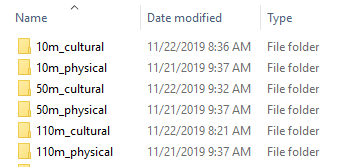
Go to their downloads page, "download all vector themes as SHP (374MB)", and extract the zip. You won't need all the files, but it's easiest to download them all ... and who knows, you might find a use for them later! Here's a listing of the folders in the extracted zip:

Side Trip

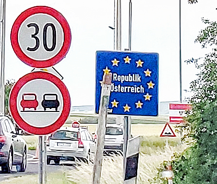
I often go on a little side-trip in my blog posts, and show one of my friends' photos. This time it's a picture my friend Eva made while traveling around Europe. What country is this Republik Österreich? Perhaps we can use one of my maps to help find out!

World Map

Let's start with the world map, containing country borders. Here's the basic code to import the shapefile. After some experimentation, I decided that the shapefile with '50m' resolution seemed about right - this is their middle resolution version of the map (10m is higher resolution, and 110m is lower resolution). Here's the main proc mapimport that reads the shapefile into a SAS dataset. You can see all the rest of the code in world.sas.

proc mapimport out=world
datafile="D:\Public\naturalearthdata\50m_cultural\ne_50m_admin_0_countries_lakes.shp";
run;

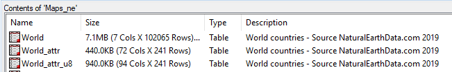
I rename some variables (for example, I change name to country, and x/y to long/lat), sort the data by country, gproject it to add a projected x/y, greduce it to add a density variable, order the variables/columns in a logical way in the dataset, and add a dataset label. I also separate out the 'attribute' data from the map dataset, and store it in a world_attr dataset (this makes it much smaller and more efficient use of space). I also create a world_attr_u8 dataset with the country names translated to several other languages (note that you must run your SAS session with utf8 encoding to create, and utilize this dataset). It took the job about 7 seconds to run on my laptop.

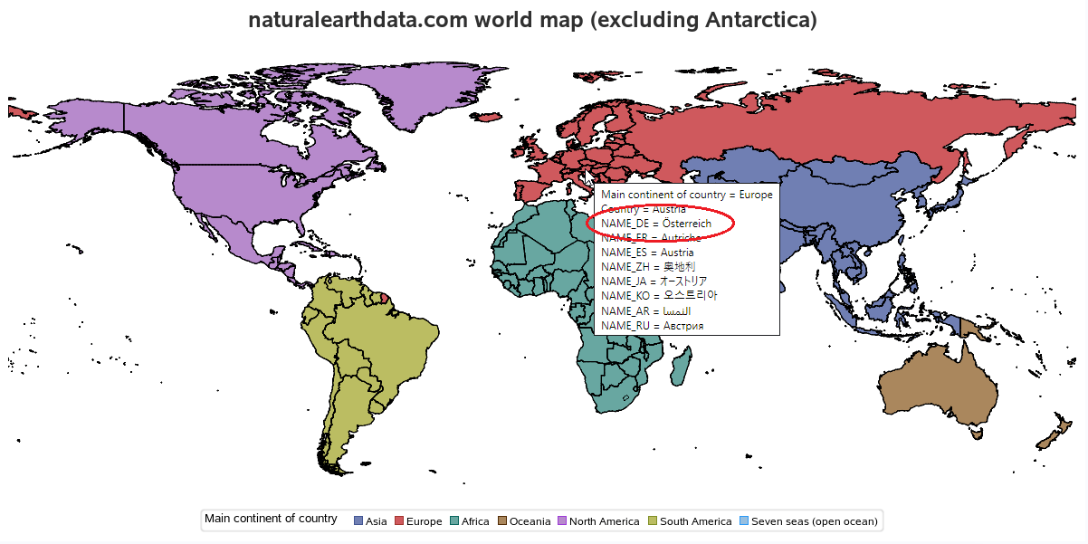
Here's what the world map looks like, just plotting the continent names as my response/color data (you'll likely have something a little more exciting to plot!) Notice the translated country names in the mouse-over text - now you can see that Österreich is what they call Austria in German. Note that specifying custom mouse-over text is a new SGmap feature in SAS Viya 3.5.

Individual Country Maps

For the individual country maps, I go with the higher-resolution '10m' maps, at the 'admin 1' level (these maps show 1 level below country - often called state or province). I first import the shapefile for the whole world at this level:

proc mapimport out=mymap
datafile="D:\Public\naturalearthdata\10m_cultural\ne_10m_admin_1_states_provinces_lakes.shp";
run;

And then loop through all the countries, and call a macro to subset that country out of the world map.

data _null_; set loopdata;
call execute('%do_one('|| dataset_name ||', '|| projection ||');');
run;

Here's basically what the macro does. It loops through the 251 countries, creating the map, _attr, and _attr_u8 dataset for each one. The job runs on my laptop in a little over 6 minutes (click here to download the whole country.sas program). Note that I haven't spent a lot of time on this code, and you will likely be able to make improvements to it.

%macro do_one(name3, proj);
/* subset the map for this country */
/* process the map (rename variables, gproject, greduce, etc) */
/* save the map in a permanent libname */
%mend;

The screen-capture below shows some examples of country datasets. Notice that I use the 3-character country abbreviation in the names ('aus' is for Australia).

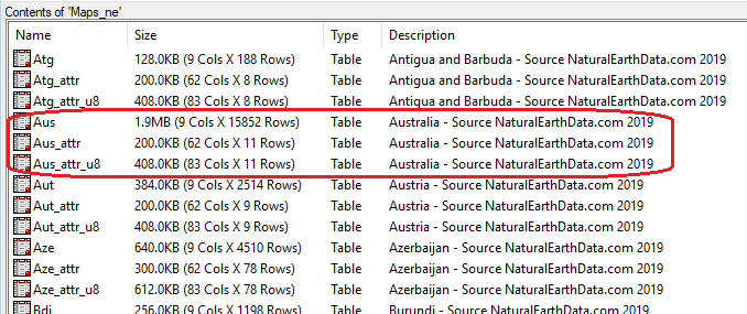
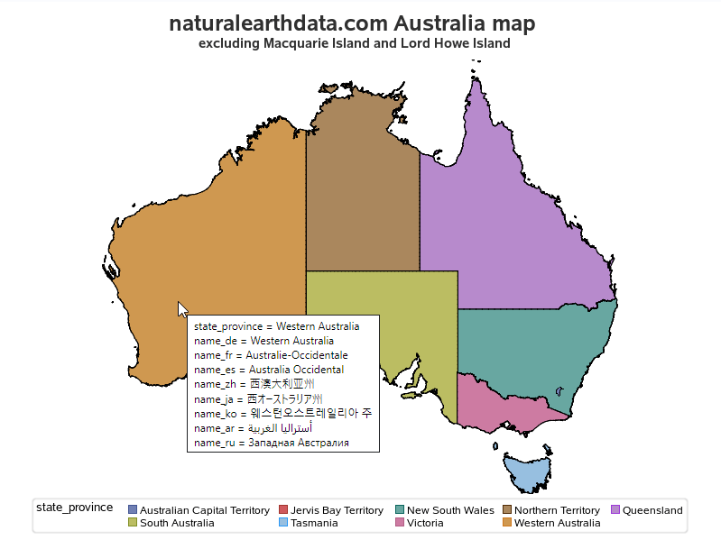
Here's what the Australia map looks like. Notice that I'm using the aus_attr_u8 file, with the names of the areas translated into different languages (again, using the new sgmap tip= feature, to specify extra variables to put in the mouse-over text, available in SAS Viya 3.5).

US State Map

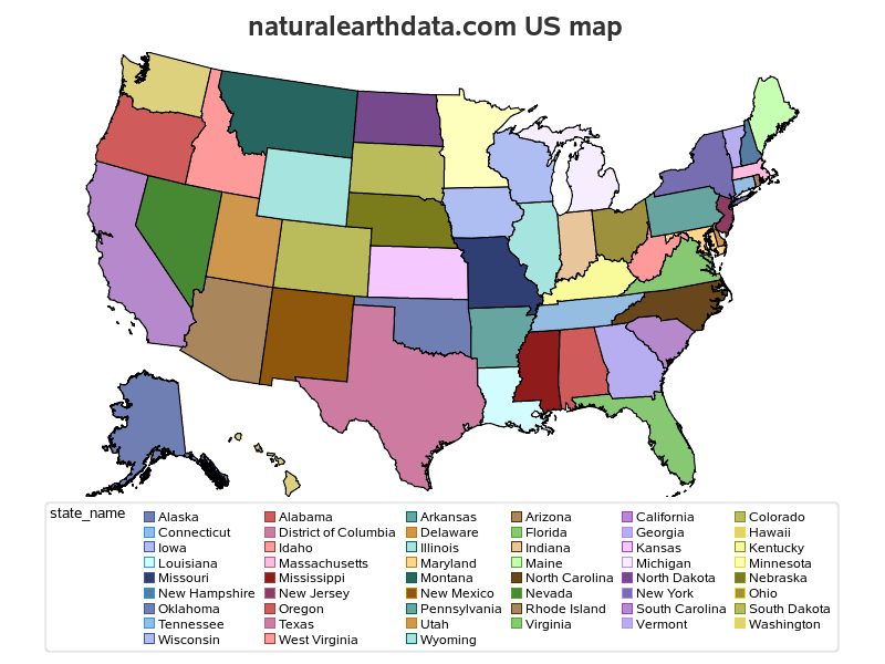
Although it is often preferable to view maps with all the areas in their proper geographical locations, there is a long tradition of moving & resizing Alaska and Hawaii so they can be easily seen on the same page as the contiguous 48 US states. In SAS/Graph, we have such a map called maps.us (or mapsgfk.us). Therefore I decided to write some code to similarly derive such a map from the NaturalEarth usa map.

I grab a copy of maps_ne.usa, break it into 3 separate datasets (one for the contiguous US states, one for Alaska, and one for Hawaii). I gproject each one separately, and then resize & move the coordinates for Alaska & Hawaii. And finally, put the 3 pieces back together in one dataset, which is very similar to the old maps.us. This job took about 1 second to run on my laptop, and you can see all the nitty-gritty details in us.sas.

Here's an example, just coloring each state by the state name (again, your data will hopefully be much more exciting!)

proc sgmap mapdata=maps_ne.us maprespdata=maps_ne.us_attr;
choromap state_name / mapid=statecode tip=(state statecode state_name);
run;

Recap

Here are those three SAS jobs again, to import the NaturalEarth shapefiles and populate your maps_ne library with your maps: world.sas, country.sas, and us.sas. If you don't have a SAS/Graph license (and therefore don't have the mapsgfk library of maps), then these can provide alternative maps for you to use with SGmap. I haven't spent a lot of time writing/testing these programs, therefore you are likely to find various ways to improve them!