A previous article shows how to construct an empirical cumulative distribution function (ECDF) for univariate data by using PROC UNIVARIATE or in the SAS IML language. The ECDF is a tool for visualizing the distribution of a sample and is helpful for estimating quantiles in the data.

In statistics, we assume that a sample is a random draw from an underlying distribution. Therefore, an ECDF has a sampling variability. As with other point estimates in statistics, you can construct a confidence band for the ECDF. The confidence band assumes that the samples are drawn randomly and independently from a population. If so, the true CDF of the population is entirely within the confidence bands for 95% of random samples.

This article shows how to use SAS to create a Kolmogorov confidence band for the ECDF. The Kolmogorov is nonparametric, which means it does not assume that the data is generated from some well-known parametric distribution such as Normal, exponential, beta, Weibull, and so forth.

The Kolmogorov confidence bands for an ECDF

One method for constructing confidence bands for an ECDF uses the Kolmogorov-Smirnov (K-S) test statistic, often denoted as D. As shown in a previous article, the K-S statistic measures the maximum absolute distance between the ECDF and the true CDF. By using the asymptotic distribution of the K-S statistic, you can calculate a 95% confidence envelope. The mathematics behind building the confidence band is presented in lecture notes from Pennsylvania State University and in lecture notes by Charles Geyer at U. MN.

To construct the 95% K-S confidence bands, you need the critical value of the Kolmogorov distribution. As noted in a previous article about critical values for the K-S statistic, the two-sided 95% critical value for the asymptotic K-S distribution is approximately 1.36. (More precisely, 1.358099.) The width of the confidence band at a point on the ECDF is the critical value divided by the square root of the sample size: D_crit/√n. Because probabilities cannot be less than 0 or greater than 1, the confidence bands are truncated at these values. (Note: for small samples and for other significance levels, you can use a SAS IML program to compute the exact critical values for any significance level.)

The following SAS IML program calculates a 95% confidence band for the ECDF of the Strength variable on the Cord data set. The program uses the ECDF module from the previous post, and the data from the Cord data set (N=50), which is defined in the same article. So, define the data set and STORE the ECDF function before running the following program.

/* Before running this program in SAS 9.4, define and STORE the ECDF function from 
   https://blogs.sas.com/content/iml/2026/05/26/create-ecdf.html 
   Also define the CORD data set from that blog post. */
proc iml;
load module=(ECDF);
 
/* The asymptotic 95th percentile of the K-S distribution is 1.358099.
   See https://blogs.sas.com/content/iml/2019/05/20/critical-values-kolmogorov-test.html
   or the lecture notes from Charles J. Geyer at U. MN. at
   https://www.stat.umn.edu/geyer/5601/examp/kolmogorov.html
*/
ks_crit = 1.358099;
 
/* read the data for the ECDF */
use Cord;  read all var "Strength" into x;  close;
 
/* evaluate the ECDF at all data points */
call sort(x);
ecdf = ECDF(x);
n = countn(x);   /* count the nonmissing values */
 
/* Compute the standard error for the K-S bands */
SE_KS = ks_crit / sqrt(n);
 
/* construct upper and lower 95% CI bands centered on the ECDF.
   The >< operator returns the minimum, ensuring the max value is 1.
   The <> operator returns the maximum, ensuring the min value is 0.
   See https://blogs.sas.com/content/iml/2026/02/04/clip-values.html */
CL95_Upper = (ecdf + SE_KS) >< 1;
CL95_Lower = (ecdf - SE_KS) <> 0;
 
create ECDF_bands var {"x" "ECDF" "CL95_Upper" "CL95_Lower" };
  append;
close;
QUIT;
 
/* Graph the step functions by using PROC SGPLOT */
title "Empirical CDF and 95% Confidence Bands";
proc sgplot data=ECDF_bands noautolegend;
   label x="Breaking Strength (psi)" ECDF="Cumulative Proportion";
   step x=X y=ECDF / lineattrs=(thickness=2);
   step x=X y=CL95_Lower / lineattrs=(color=gray);
   step x=X y=CL95_Upper / lineattrs=(color=gray);
   xaxis grid label="x";
   yaxis grid min=0 offsetmin=0.03;
run;

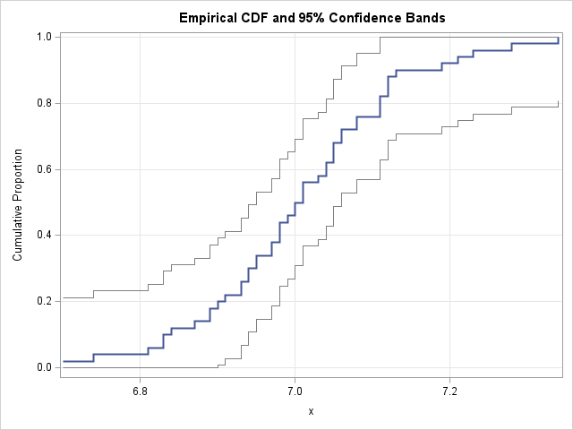
The SGPLOT procedure overlays three separate STEP statements to display the ECDF, the 95% lower band, and the 95% upper band. I did not use the BAND statement (which creates a filled region) because it is designed for continuous curves. You could use a POLYGON statement if you need to display a filled region. I leave that as an exercise.

How to interpret the confidence limits

The K-S bands are simultaneous confidence bands, not pointwise confidence intervals. There is a big difference!

If these were pointwise intervals, a 95% interval at a specific value like x = 7 would mean, "the true CDF value at x = 7 is within the vertical range for 95% of random samples." However, the interpretation is different for simultaneous bands. The bands indicate that, in 95% of random samples, the entire CDF curve for the population will lie between these upper and lower step functions for all values of x. This is a stronger statement, which is why the Kolmogorov bands are generally wide for small samples. The Cord data set has 50 observations, so wide bands.

Incidentally, it is straightforward to wrap the computation in this section into a SAS IML function that computes the confidence bands for any ECDF. Furthermore, you can compute the bands for any confidence level, not just for the 95% level. The Appendix defines a SAS IML function that computes Kolmogorov confidence bands for an ECDF for any confidence level.

Advantages and disadvantages of Kolmogorov bands

Some advantages of Kolmogorov bands include:

• Nonparametric: The Kolmogorov bands do not assume any specific distribution for the data. (For example, it is not assumed to be normal.) Thus, the bands are very general.
• Easy to Compute: The K-S bands are easy to compute. You merely need to add and subtract a term that depends on the sample size and the critical value of the Kolmogorov D statistic.

Kolmogorov bands have a few statistical shortcomings:

• Constant Width: Before the limits are truncated at 0 and 1, the K-S bands have the same vertical width at the center of the data as they do in the tails. In reality, the variance of an ECDF approaches 0 at the tails (because the CDF must exactly reach 0 and 1). Consequently, K-S bands are overly conservative (too wide) in the tails.
• Continuous Assumption: The critical values of the standard K-S test assume the underlying population distribution is perfectly continuous. If your data contains many tied values (perhaps due to rounding or limitations of the instruments used to measure the data), the bands will be conservative, meaning the true coverage probability might be higher than the nominal 95%.

Summary

Plotting an ECDF is one way to summarize univariate data. Like any statistic, the ECDF has uncertainty due to random sampling. You can use the asymptotic distribution of the Kolmogorov-Smirnov statistic to calculate simultaneous 95% confidence bands for the ECDF. Thus, you can overlay confidence bands on an ECDF. The K-S bands are somewhat conservative at the extremes of the data, but they are a classic, nonparametric, and easily interpretable way to visualize uncertainty in an ECDF.

The ECDF is a valuable tool for theoretical purposes and for ECDF-based goodness-of-fit tests. However, when comparing the data to a parametric distribution, many practitioners prefer Q-Q plots. Q-Q plots are preferred because it is easier to judge whether points fall on a straight line than it is to see the difference between two S-shaped curves. You can use the inverse-CDF transformation to map the K-S bands from the ECDF plot onto a Q-Q plot. I will demonstrate this transformation in a future article.

Appendix: A SAS IML function that computes Kolmogorov confidence bands for an ECDF

It is straightforward to wrap the computation in this article into a SAS IML function. The following program defines a function named ECDF_KSCL. It computes the K-S confidence bands for any confidence level in the range [0.75, 0.99], in increments of 0.01. If you pass in a level such as 0.975, it will be rounded to the nearest 0.01. The critical values for the K-S statistic were computed by using an IML program similar to the one in the lecture notes by Charles Geyer at U. MN.

proc iml;
/* Compute the Kolmogorov-Smirnov confidence bands for a given ECDF.
   The CL parameter specifies the confidence level, which defaults to 0.95.
   The CL parameter should be in the range [0.75, 0.99]. */
start ECDF_KSCL(_ECDF, CL=0.95);
   ECDF = colvec(_ECDF);      /* ensure column vector */
   n = countn(ECDF);          /* count the nonmissing values */
   KS_band = j(nrow(ECDF), 2, .);
   /* Enter a pre-tabulated set of critical values for confidence levels */
   dAlpha = 0.01;
   alpha = do(0.01, 0.25, dAlpha);
   conf_level = round(1 - alpha, dAlpha);
   ks_crit = { 1.6276236 1.517427 1.4490862 1.3985734 1.3580986 
               1.3241093 1.2946745 1.2686236 1.2451911 1.2238479 
               1.2042125 1.1860005 1.1689938 1.1530214 1.1379465 
               1.1236583 1.110065 1.0970904 1.0846701 1.0727492 
               1.0612805 1.0502232 1.0395418 1.0292048 1.0191847 };
   j = loc( conf_level = round(CL, dAlpha) );
   if ncol(j)=0 then do;
      print "ERROR in ECDF_KSCL: The confidence level must be between 0.75 and 0.99";
      return( KS_band );
   end;
   /* Compute the standard error for the K-S bands */
   SE_KS = ks_crit[j] / sqrt(n);
 
   /* construct upper and lower 95% CI bands centered on the ECDF.
      The >< operator returns the minimum, ensuring max value is 1.
      The <> operator returns the maximum, ensuring min value is 0.
      See https://blogs.sas.com/content/iml/2026/02/04/clip-values.html */
   CL_Upper = (ECDF + SE_KS) >< 1;
   CL_Lower = (ECDF - SE_KS) <> 0;
   KS_band = CL_Lower || CL_Upper;
   return KS_Band;
finish;
store module=(ECDF_KSCL);
QUIT;
 
/* Test the ECDF_KSCL function */
proc iml;
load module=(ECDF ECDF_KSCL);
 
/* read the data for the ECDF */
use Cord;  read all var "Strength" into x;  close;
/* evaluate the ECDF at all data points */
call sort(x);
ecdf = ECDF(x);
CL = ECDF_KSCL(ecdf, 0.90); /* get bands for any confidence levels in [0.75, 0.99] */
CL_Lower = CL[,1];
CL_Upper = CL[,2];
create ECDF_bands var {"x" "ECDF" "CL_Lower" "CL_Upper" };
  append;
close;
QUIT;
 
/* Graph the step functions by using PROC SGPLOT */
title "Empirical CDF and 90% Confidence Bands";
proc sgplot data=ECDF_bands noautolegend;
   label x="Breaking Strength (psi)" ECDF="Cumulative Proportion";
   step x=X y=ECDF / lineattrs=(thickness=2);
   step x=X y=CL_Lower / lineattrs=(color=gray);
   step x=X y=CL_Upper / lineattrs=(color=gray);
   xaxis grid label="x";
   yaxis grid min=0 offsetmin=0.03;
run;