Have you ever run a statistical test to determine whether data are normally distributed? If so, you have probably used Kolmogorov's D statistic. Kolmogorov's D statistic (also called the Kolmogorov-Smirnov statistic) enables you to test whether the empirical distribution of data is different than a reference distribution. The reference distribution can be a probability distribution or the empirical distribution of a second sample. Most statistical software packages provide built-in methods for computing the D statistic and using it in hypothesis tests. This article discusses the geometric meaning of the Kolmogorov D statistic, how you can compute it in SAS, and how you can compute it "by hand."

This article focuses on the case where the reference distribution is a continuous probability distribution, such as a normal, lognormal, or gamma distribution. The D statistic can help you determine whether a sample of data appears to be from the reference distribution. Throughout this article, the word "distribution" refers to the cumulative distribution.

What is the Kolmogorov D statistic?

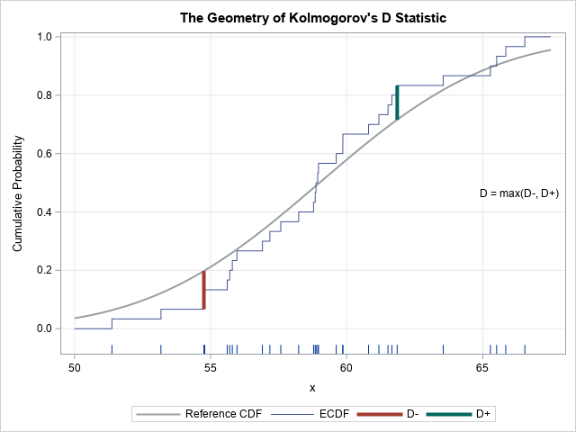
The letter "D" stands for "distance." Geometrically, D measures the maximum vertical distance between the empirical cumulative distribution function (ECDF) of the sample and the cumulative distribution function (CDF) of the reference distribution. As shown in the adjacent image, you can split the computation of D into two parts:

• When the reference distribution is above the ECDF, compute the statistic D^– as the maximal difference between the reference distribution and the ECDF. Because the reference distribution is monotonically increasing and because the empirical distribution is a piecewise-constant step function that changes at the data values, the maximal value of D^– will always occur at a right-hand endpoint of the ECDF.
• When the reference distribution is below the ECDF, compute the statistic D⁺ as the maximal difference between the ECDF and the reference distribution. The maximal value of D⁺ will always occur at a left-hand endpoint of the ECDF.

The D statistic is simply the maximum of D^– and D⁺.

You can compare the statistic D to critical values of the D distribution, which appear in tables. If the statistic is greater than the critical value, you reject the null hypothesis that the sample came from the reference distribution.

How to compute Kolmogorov's D statistic in SAS?

In SAS, you can use the HISTOGRAM statement in PROC UNIVARIATE to compute Kolmogorov's D statistic for many continuous reference distributions, such as the normal, beta, or gamma distributions. For example, the following SAS statements simulate 30 observations from a N(59, 5) distribution and compute the D statistic as the maximal distance between the ECDF of the data and the CDF of the N(59, 5) distribution:

/* parameters of reference distribution: F = cdf("Normal", x, &mu, &sigma) */
%let mu    = 59;
%let sigma =  5;
%let N     = 30;
 
/* simulate a random sample of size N from the reference distribution */
data Test;
call streaminit(73);
do i = 1 to &N;
   x = rand("Normal", &mu, &sigma);
   output;
end;
drop i;
run;
 
proc univariate data=Test;
   ods select Moments CDFPlot GoodnessOfFit;
   histogram x / normal(mu=&mu sigma=&sigma) vscale=proportion;  /* compute Kolmogov D statistic (and others) */
   cdfplot x / normal(mu=&mu sigma=&sigma) vscale=proportion;    /* plot ECDF and reference distribution */
   ods output CDFPlot=ECDF(drop=VarName CDFPlot);                /* for later use, save values of ECDF */
run;

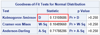
The computation shows that D = 0.131 for this simulated data. The plot at the top of this article shows that the maximum occurs for a datum that has the value 54.75. For that observation, the ECDF is farther away from the normal CDF than at any other location.

The critical value of the D distribution when N=30 and α=0.05 is 0.2417. Since D < 0.2417, you should not reject the null hypothesis. It is reasonable to conclude that the sample comes from the N(59, 5) distribution.

Although the computation is not discussed in this article, you can use PROC NPAR1WAY to compute the statistic when you have two samples and want to determine if they are from the same distribution. In this two-sample test, the geometry is the same, but the computation is slightly different because the reference distribution is itself an ECDF, which is a step function.

Compute Kolmogorov's D statistic manually

Although PROC UNIVARIATE in SAS computes the D statistic (and other goodness-of-fit statistics) automatically, it is not difficult to compute the statistic from first principles in a vector language such as SAS/IML.

The key is to recall that the ECDF is a piecewise constant function that changes heights at the value of the observations. If you sort the data, the height at the i_th sorted observation is i / N, where N is the sample size. The height of the ECDF an infinitesimal distance before the i_th sorted observation is (i – 1)/ N. These facts enable you to compute D^– and D⁺ efficiently.

The following algorithm computes the D statistic:

1. Sort the data in increasing order.
2. Evaluate the reference distribution at the data values.
3. Compute the pairwise differences between the reference distribution and the ECDF.
4. Compute D as the maximum value of the pairwise differences.

The following SAS/IML program implements the algorithm:

/* Compute the Kolmogorov D statistic manually */
proc iml;
use Test;  read all var "x";  close;
N = nrow(x);                         /* sample size */
call sort(x);                        /* sort data */
F = cdf("Normal", x, &mu, &sigma);   /* CDF of reference distribution */
i = T( 1:N );                        /* ranks */
Dminus = F - (i-1)/N;
Dplus = i/N - F;
D = max(Dminus, Dplus);              /* Kolmogorov's D statistic */
print D;

The D statistic matches the computation from PROC UNIVARIATE.

The SAS/IML implementation is very compact because it is vectorized. By computing the statistic "by hand," you can perform additional computations. For example, you can find the observation for which the ECDF and the reference distribution are farthest away. The following statements find the index of the maximum for the Dminus and Dplus vectors. You can use that information to find the value of the observation at which the maximum occurs, as well as the heights of the ECDF and reference distribution. You can use these values to create the plot at the top of this article, which shows the geometry of the Kolmogorov D statistic:

/* compute locations of the maximum D+ and D-, then plot with a highlow plot */
i1 = Dminus[<:>];  i2 = Dplus [<:>];              /* indices of maxima */
/* Compute location of max, value of max, upper and lower curve values */
x1=x[i1];  v1=DMinus[i1];  Low1=(i[i1]-1)/N;  High1=F[i1]; 
x2=x[i2];  v2=Dplus [i2];  Low2=F[i2];        High2=i[i2]/N; 
Result = (x1 || v1 || Low1 || High1) // (x2 || v2 || Low2 || High2);
print Result[c={'x' 'Value' 'Low' 'High'} r={'D-' 'D+'} L='Kolmogorov D'];

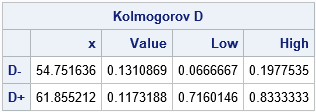
The observations that maximize the D^– and D⁺ statistics are x=54.75 and x=61.86, respectively. The value of D^– is the larger value, so that is the value of Kolmogorov's D.

For completeness, the following statement show how to create the graph at the top of this article. The HIGHLOW statement in PROC SGPLOT is used to plot the vertical line segments that represent the D^– and D⁺ statistics.

create KolmogorovD var {x x1 Low1 High1 x2 Low2 High2}; append; close;
quit;
 
data ALL;
   set KolmogorovD ECDF;   /* combine the ECDF, reference curve, and the D- and D+ line segments */
run;
 
title "Kolmogorov's D Statistic";
proc sgplot data=All;
   label CDFy = "Reference CDF" ECDFy="ECDF";
   xaxis grid label="x";
   yaxis grid label="Cumulative Probability" offsetmin=0.08;
   fringe x;
   series x=CDFx Y=CDFy / lineattrs=GraphReference(thickness=2) name="F";
   step x=ECDFx Y=ECDFy / lineattrs=GraphData1 name="ECDF";
   highlow x=x1 low=Low1 high=High1 / 
           lineattrs=GraphData2(thickness=4) name="Dm" legendlabel="D-";
   highlow x=x2 low=Low2 high=High2 / 
           lineattrs=GraphData3(thickness=4) name="Dp" legendlabel="D+";
   keylegend "F" "ECDF" "Dm" "Dp";
run;

Concluding thoughts

Why would anyone want to compute the D statistic by hand if PROC UNIVARIATE can compute it automatically? There are several reasons:

• Understanding: When you compute a statistic manually, you are forced to understand what the statistic means and how it works.
• Efficiency: When you run PROC UNIVARIATE, it computes many statistics (mean, standard deviation, skewness, kurtosis,...), many goodness-of-fit tests (Kolmogorov-Smirnov, Anderson-Darling, and Cramér–von Mises), a histogram, and more. That's a lot of work! If you are interested only in the D statistic, why needlessly compute the others?
• Generalizability: You can compute quantities such as the location of the maximum value of D^– and D⁺. You can use the knowledge and experience you've gained to compute related statistics.