Recently I wrote about how to compute the Kolmogorov D statistic, which is used to determine whether a sample has a particular distribution. One of the beautiful facts about modern computational statistics is that if you can compute a statistic, you can use simulation to estimate the sampling distribution of that statistic. That means that instead of looking up critical values of the D statistic in a table, you can estimate the critical value by using empirical quantiles from the simulation.

This is a wonderfully liberating result! No longer are we statisticians constrained by the entries in a table in the appendix of a textbook. In fact, you could claim that modern computation has essentially killed the standard statistical table.

Obtain critical values by using simulation

Before we compute anything, let's recall a little statistical theory. If you get a headache thinking about null hypotheses and sampling distributions, you might want to skip the next two paragraphs!

When you run a hypothesis test, you compare a statistic (computed from data) to a hypothetical distribution (called the null distribution). If the observed statistic is way out in a tail of the null distribution, you reject the hypothesis that the statistic came from that distribution. In other words, the data does not seem to have the characteristic that you are testing for. Statistical tables use "critical values" to designate when a statistic is in the extreme tail. What is a "critical value"? A critical value is a quantile of the null distribution; if the observed statistic is greater than the critical value, then the statistic is in the tail. (Technically, I've described a one-tailed test.)

One of the uses for simulation is to approximate the sampling distribution of a statistic when the true distribution is not known or is known only asymptotically. You can generate a large number of samples from the null hypothesis and compute the statistic on each sample. The distribution of the statistics approximates the true sampling distribution (under the null hypothesis) so you can use the quantiles to estimate the critical values of the null distribution.

Critical values of the Kolmogorov D distribution

You can use simulation to estimate the critical value for the Kolmogorov-Smirnov statistical test for normality, which is sometimes abbreviated as the "KS test." For the data in my previous article, the null hypothesis is that the sample data follow a N(59, 5) distribution. The alternative hypothesis is that they do not. The previous article computed a KS test statistic of D = 0.131 for the data (N = 30). If the null hypothesis is true, is that an unusual value to observe? Let's simulate 40,000 samples of size N = 30 from N(59,5) and compute the D statistic for each. Rather than use PROC UNIVARIATE, which computes dozens of statistics for each sample, you can use the SAS/IML computation from the previous article, which is very fast. The following simulation runs in a fraction of a second.

/* parameters of reference distribution: F = cdf("Normal", x, &mu, &sigma) */
%let mu    = 59;
%let sigma =  5;
%let N     = 30;
%let NumSamples = 40000;
 
proc iml;
call randseed(73);
N = &N;
i = T( 1:N );                           /* ranks */
u = i/N;                                /* ECDF height at right-hand endpoints */
um1 = (i-1)/N;                          /* ECDF height at left-hand endpoints  */
 
y = j(N, &NumSamples, .);               /* columns of Y are samples of size N */
call randgen(y, "Normal", &mu, &sigma); /* fill with random N(mu, sigma)      */
D = j(&NumSamples, 1, .);               /* allocate vector for results        */
 
do k = 1 to ncol(y);                    /* for each sample:                   */
   x = y[,k];                           /*    get sample x ~ N(mu, sigma)     */
   call sort(x);                        /*    sort sample                     */
   F = cdf("Normal", x, &mu, &sigma);   /*    CDF of reference distribution   */
   D[k] = max( F - um1, u - F );        /*    D = max( D_minus, D_plus )      */
end;
 
title "Monte Carlo Estimate of Sampling Distribution of Kolmogorov's D Statistic";
title2 "N = 30; N_MC = &NumSamples";
call histogram(D) other=
     "refline 0.131 / axis=x label='Sample D' labelloc=inside lineattrs=(color=red);";

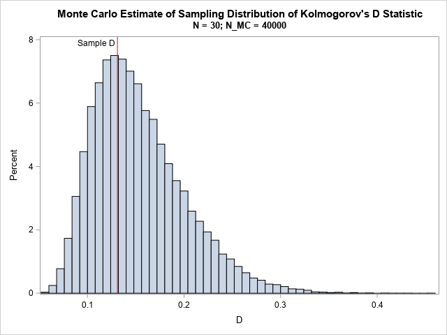
The KS test statistic is right smack dab in the middle of the null distribution, so there is no reason to doubt that the sample is distributed as N(59, 5).

How big would the KS test statistic need to be to be considered extreme? To test the hypothesis at the α significance level, you can compute the 1 – α quantile of the null distribution. The following statements compute the critical value for α = 0.05 and N = 30:

/* estimate critical value as the 1 - alpha quantile */
alpha = 0.05;
call qntl(Dcrit_MC, D, 1-alpha);
print Dcrit_MC;

The estimated critical value for a sample of size 30 is 0.242. This compares favorably with the exact critical value from a statistical table, which gives D_crit = 0.2417 for N = 30.

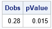
You can also use the null distribution to compute a p value for an observed statistic. The p value is estimated as the proportion of statistics in the simulation that exceeds the observed value. For example, if you observe data that has a D statistic of 0.28, the estimated p value is obtained by the following statements:

Dobs = 0.28;                        /* hypothetical observed statistic */
pValue = sum(D >= Dobs) / nrow(D);  /* proportion of distribution values that exceed D0 */
print Dobs pValue;

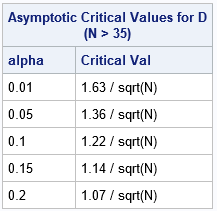
This same technique works for any sample size, N, although most tables critical values only for all N ≤ 30. For N > 35, you can use the following asymptotic formulas, developed by Smirnov (1948), which depend only on α:

The Kolmogorov D statistic does not depend on the reference distribution

It is reasonable to assume that the results of this article apply only to a normal reference distribution. However, Kolmogorov proved that the sampling distribution of the D statistic is actually independent of the reference distribution. In other words, the distribution (and critical values) are the same regardless of the continuous reference distribution: beta, exponential, gamma, lognormal, normal, and so forth. That is a surprising result, which explains why there is only one statistical table for the critical values of the Kolmogorov D statistic, as opposed to having different tables for different reference distributions.

In summary, you can use simulation to estimate the critical values for the Kolmogorov D statistic. In a vectorized language such as SAS/IML, the entire simulation requires only about a dozen statements and runs extremely fast.