Create and graph the ECDF function in SAS

The empirical cumulative distribution function (ECDF) is an important tool in statistics. It is one of several plots you can use to visualize the shape of a data distribution. It is not used as often as the histogram, the kernel density estimate, and the box plot, but it is essential to visualize ECDF-based hypothesis tests that assess whether the data might have come from a specified distribution.

This article shows how to construct and plot an ECDF in SAS. The easy way is to use PROC UNIVARIATE. However, for certain data analysis applications, it is useful to be able to call a function in the SAS IML matrix language that manually evaluates the ECDF. The ECDF function was added to the SAS IML language in the 2025.01 release of SAS Viya. For customers who are still on SAS 9.4, this article provides a similar ECDF function that you can use.

What is an ECDF?

Given a set of univariate data x₁ ≤ x₂ ≤ ... ≤ x_n, the empirical distribution function (ECDF) is the step function defined by:
F(t) = (number of data values ≤ t) / n

The ECDF is a piecewise-constant function that is flat on each half-open interval [x_i, x_i+1). At each unique data value, it increases by an amount proportional to the frequency of data at that value.

The ECDF in PROC UNIVARIATE

SAS provides the CDFPLOT statement in PROC UNIVARIATE, which computes and displays the ECDF and optionally overlays the CDF of a specified probability distribution. For example, the PROC UNIVARIATE documentation includes data about the breaking strength (in PSI) for 50 fiber-optic cords:

data Cord;
   label Strength="Breaking Strength (psi)";
   input Strength @@;
datalines;
6.94 6.97 7.11 6.95 7.12 6.70 7.13 7.34 6.90 6.83
7.06 6.89 7.28 6.93 7.05 7.00 7.04 7.21 7.08 7.01
7.05 7.11 7.03 6.98 7.04 7.08 6.87 6.81 7.11 6.74
6.95 7.05 6.98 6.94 7.06 7.12 7.19 7.12 7.01 6.84
6.91 6.89 7.23 6.98 6.93 6.83 6.99 7.00 6.97 7.01
;
 
title 'Cumulative Distribution Function of Breaking Strength';
proc univariate data=Cord noprint;
   cdfplot Strength / odstitle = title;
run;

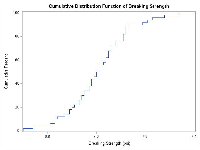
From the plot, you can see that there is about a 50% chance that a random fiber-optic cord will break if subjected to 7.0 PSI of stress. If the stress is kept below 6.9 PSI, there is only a 20% chance of random cord will break. The graph can be improved to answer questions like these by using the STATREF= option on the CDFPLOT statement to add vertical reference lines at the data value that correspond to arbitrary percentiles. For example, the option statref=P 10 Q1 Q2 Q3 P 90 add vertical lines at the 10th, 25th, 50th, 75th, and 90th percentiles of the data.

In addition to displaying the ECDF, the CDFPLOT statement enables you to overlay the theoretical CDF of common probability distributions. This is useful for visualizing ECDF-based hypothesis tests. For example, the Kolmogorov-Smirnov (K-S) test for normality uses the largest vertical gap between the ECDF and the hypothesized CDF to construct a test statistic. If you add the NORMAL option to the CDFPLOT statement, you can visualize the K-S test and other ECDF-based goodness-of-fit tests for normality.

How to construct an ECDF manually

When conducting a simulation study, a bootstrap analysis, or exploring ECDF-based statistics, it is convenient to compute ECDF values in SAS IML. To construct the ECDF manually, do the following:

Find the unique values in the data and the number of observations for each unique value. In SAS IML, you can use the TABULATE function for that.
Since the ECDF is a piecewise constant function that steps up at these locations, use these unique values as the endpoints of bins. You can use the BIN function for that.
For each bin, associate the value of the ECDF function at the left endpoint of the bin. Since the ECDF is a piecewise constant function that increases at these locations, this tells you the values of the ECDF for any point in any bin.
For points that are outside of any bin, the ECDF is either 0 or 1. If t is less than the smallest data value, ECDF(t) = 0. If t is greater than or equal to the largest data value, then ECDF(t) = 1.

In SAS Viya, the ECDF function is supported natively by the SAS IML language. For customers who are still on SAS 9.4, the following function manually implements the basic ECDF algorithm:

proc iml;
/* Compute the empirical distribution function (ECDF) if a column vector of data.
   Optionally, evaluate the ECDF at values in a column vector, t. 
   If t is not specified, use t=x. 
   SYNTAX:
     y = ECDF(x); 
     t = T( do( min(x), max(x), (max(x)-min(x))/100 ) );
     y = ECDF(x, t); 
*/
start ECDF(_x, _t=);
    x = colvec(_x);      /* ensure a column vector */
    /* Tabulate the unique values of x.
       levels = unique sorted elements of x
       freq = number of duplicates for each level */
    call tabulate(levels, freq, x);
    levels = colvec(levels);
    freq = colvec(freq);
    y = cusum(freq) / sum(freq);
 
    if isSkipped(_t) then
       t = x;
    else
       t = colvec(_t);      /* ensure column vector */
    /* build a step function by assigning t to different bins, using levels as endpoints */
    bins = bin(t, levels);
 
    /* assign ECDF[i] for nonmissing bins */
    ecdf = j(nrow(t), 1, .);    /* initialize ECDF to missing */
    idx = loc(bins ^= .);
    if ncol(idx) > 0 then
        ecdf[idx] = y[ bins[idx] ];
 
    /* Three reasons bins[i] could be a missing value:
       1. if t[i] is missing. No need to change ECDF[i] b/c it was initialized to missing.
       2. if t[i] < min(x). Set ECDF(t[i]) = 0.
       3. if t[i] > max(x). Set ECDF(t[i]) = 1.
    */
    LT_idx = loc(t^=. & t<min(x));
    if ncol(LT_idx) > 0 then 
       ecdf[LT_idx] = 0;
    GT_idx = loc(t^=. & t>=max(x));
    if ncol(GT_idx) > 0 then 
       ecdf[GT_idx] = 1;
    return ecdf;
finish;
store module=(ECDF);
QUIT;

Let's call this function on the same data that was used by PROC UNIVARIATE earlier in this article. Suppose you want to estimate the probability that the breaking strength of a fiber optic cord is less than certain specified test values. You can read the Cord data set and call the ECDF function, as follows:

proc iml;
load module=(ECDF);
 
use Cord;
read all var "Strength" into x;
close;
 
/* estimate the probability that the breaking strength is less than 
   6.8, 6.9, 7.0, and 7.1 psi. Note that some of these values 
   are not observed data values.
*/
t = {6.8, 6.9, 7.0, 7.1};
ecdf_t = ECDF(x, t);
print t ecdf_t;

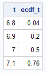
The output estimates the probability that a random cord will break when subjected to the specified stresses. About 4% will break if the stress is 6.8 PSI, whereas about 76% will break is the stress is as large as 7.1 PSI.

Notice that some of the specified locations are not data values. For each specified value, the ECDF returns an estimate of the probability that a random fiber-optic cord will break when subjected to a stress of that magnitude.

Graph the ECDF

Typically, an ECDF plot evaluates the ECDF function at the observed data values rather than arbitrary points. As discussed in a previous article, it is best to use the STEP statement in PROC SGPLOT to visualize an ECDF function.

The following IML statements sort the data, evaluate the ECDF at the data locations, and write the resulting calculations to a SAS data set. The SGPLOT procedure then visualizes the ECDF.

/* typically, an ECDF plot evaluates the ECDF at all data points */
call sort(x);
ecdf = ECDF(x);
 
create ECDF var {"x" "ECDF"}; append; close;
QUIT;
 
/* Graph a step function. See
   https://blogs.sas.com/content/iml/2016/09/06/graph-step-function-sas.html */
title "Empirical CDF";
proc sgplot data=ECDF noautolegend;
   label x="Breaking Strength (psi)" ECDF="Cumulative Proportion";
   step x=x y=ecdf;
   fringe x;
   xaxis grid label="x" offsetmin=0.05 offsetmax=0.05;
   yaxis grid min=0 offsetmin=0.03;
run;

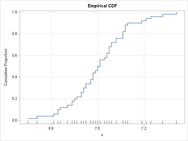
The resulting graph is similar to the one produced by PROC UNIVARIATE earlier. However, by using PROC SGPLOT, you have more freedom to enhance the plot with features such as a fringe plot, custom reference lines, grid lines, and so on. The grid lines enable you to quickly estimate that about 50% of random cords will creak if subjected to a stress of 7.0 PSI.

Summary

The empirical CDF (ECDF) is a fundamental nonparametric tool for exploring data and comparing univariate distributions. In Base SAS, PROC UNIVARIATE provides a quick and easy way to generate these plots automatically. In addition, it can be useful to be able to evaluate the ECDF function programmatically. The ECDF function was added to SAS IML in SAS Viya in Release 2025.01. For SAS 9.4 customers, this article provides a similar function.

Blogs