The Kolmogorov D distribution and exact critical values

If you have ever run a Kolmogorov-Smirnov test for normality, you have encountered the Kolmogorov D statistic. The Kolmogorov D statistic is used to assess whether a random sample was drawn from a specified distribution. Although it is frequently used to test for normality, the statistic is "distribution free" in the sense that it compares the empirical distribution to any specified distribution. I have previously written about how to interpret the Kolmogorov D statistic and how to compute it in SAS.

If you can compute a statistic, you can use simulation to approximate its sampling distribution and to approximate its critical values. Although I am a fan of simulation, in this article I show how to compute the exact distribution and critical values for Kolmogorov D statistic. The technique used in this article is from Facchinetti (2009), "A Procedure to Find Exact Critical Values of Kolmogorov-Smirnov Test."

An overview of the Facchinetti method

Suppose you have a sample of size n and you perform a Kolmogorov-Smirnov test that compares the empirical distribution to a reference distribution. You obtain the test statistic D. To know whether you should reject the null hypothesis (that the test came from the reference distribution), you need to be able to compute the probability CDF(D) = Pr(D_n ≤ D). Facchinetti shows that you can compute the probability for any D by solving a system of linear equations. If a random sample contains n observations, you can form a certain (2n+2) x (2n+2) matrix whose entries are composed of binomial probabilities. You can use a discrete heat map to display the structure of the matrix that is used in the Facchinetti method. One example is shown below. For n=20, the matrix is 42 x 42. As Facchinetti shows in Figure 6 of her paper, the matrix has a block structure, with triangular matrices in four blocks.

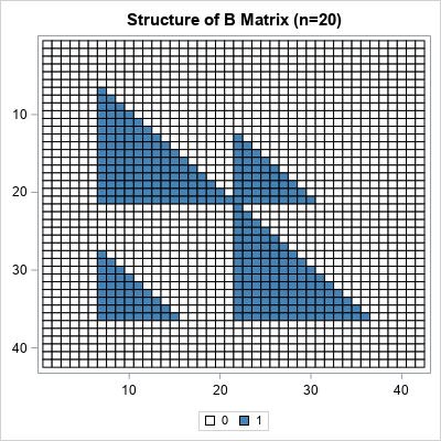
The right-hand side of the linear system is also composed of binomial probabilities. The system is singular, but you can use a generalized inverse to obtain a solution. From the solution, you can compute the probability. For the details, see Facchinetti (2009).

Facchinetti includes a MATLAB program in the appendix of her paper. I converted the MATLAB program into SAS/IML and improved the efficiency by vectorizing some of the computations. You can download the SAS/IML program that computes the CDF of the Kolmogorov D statistic and all the graphs in this article. The name of the SAS/IML function is KolmogorovCDF, which requires two arguments, n (sample size) and D (value of the test statistic).

Examples of using the CDF of the Kolmorov distribution

Suppose you have a sample of size 20. You can use a statistical table to look up the critical value of the Kolmogorov D statistic. For α = 0.05, the (two-sided) critical value for n=20 is D = 0.294. If you load and call the KolmogorovCDF function, you can confirm that the CDF for the Kolmogorov D distribution is very close to 0.95 when D=0.294:

proc iml;
load  module=KolmogorovCDF;      /* load the function that implements the Facchinetti method */
/* simple example of calling the function */
n = 20;
D = 0.29408;
cdf = KolmogorovCDF(n, D);
print n D cdf;

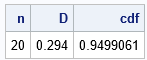
The interpretation of this result is that if you draw a random samples of size 20 from the reference distribution, there is a 5% chance that the Kolmogorov D value will exceed 0.294. A test statistic that exceeds 0.294 implies that you should reject the null hypothesis at the 0.05 significance level.

Visualize the Kolmogorov D distribution

If you can compute the CDF for one value of D, you can compute it for a sequence of D values. In this way, you can visualize the CDF curve. The following SAS/IML statements compute the CDF for the Kolmogorov D distribution when n=20 by running the computation on a sequence of D values in the open interval (0, 1):

D = do(0.01, 0.99, 0.01);             /* sequence of D values */
CDF = j(1, ncol(D), .);
do i = 1 to ncol(D);
   CDF[i] = KolmogorovCDF(n, D[i]);   /* CDF for each D */ 
end;
title "Kolmogorov CDF, n=20";
call series(D, CDF) grid={x y};       /* create a graph of the CDF */

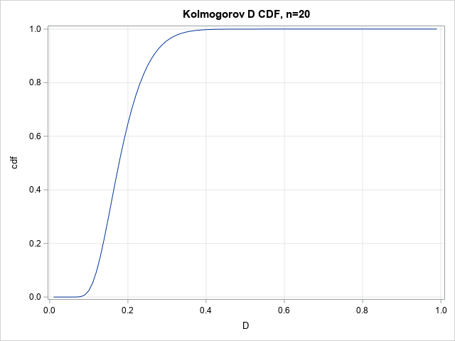
The graph enables you to read probabilities and quantiles for the D₂₀ distribution. The graph shows that almost all random samples of size 20 (drawn from the reference distribution) will have a D statistic of less than 0.4. Geometrically, the D statistic represents the largest gap between the empirical distribution and the reference distribution. A large gap indicates that the sample was probably not drawn from the reference distribution.

Visualize a family of Kolmogorov D distributions

The previous graph was for n=20, but you can repeat the computation for other values of n to obtain a family of CDF curves for the Kolmogorov D statistic. (Facchinetti writes D_n to emphasize that the statistic depends on the sample size.) The computation is available in the program that accompanies this article. The results are shown below:

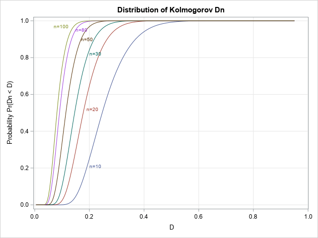
This graph enables you to estimate probabilities and quantiles for several D_n distributions.

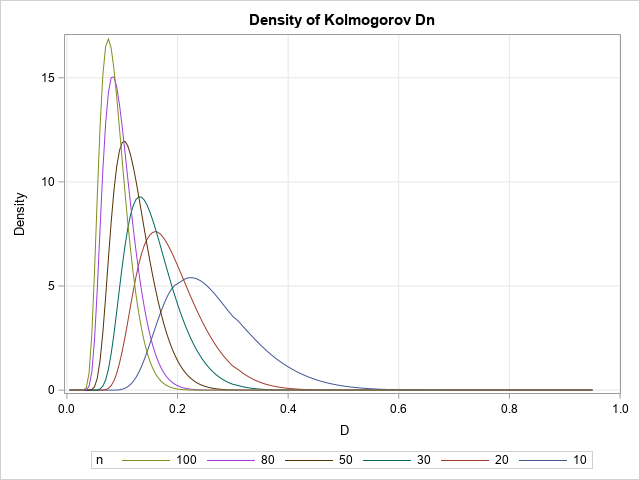
Visualize a family of density curves

Because the PDF is the derivative of the CDF, you can use a forward difference approximation of the derivative to also plot the density of the distribution. The following density curves are derived from the previous CDF curves:

A table of critical values

If you can compute the CDF, you can compute quantiles by using the inverse CDF. You can use a root-finding technique to obtain a quantile.

In the SAS/IML language, the FROOT function can find univariate roots. The critical values of the D_n statistic are usually tabulated by listing the sample size down columns and the significance level (α) or confidence level (1-α) across the columns. Facchinetti (p. 352) includes a table of critical values in her paper. The following SAS/IML statements show how to recreate the table. For simplicity, I show only a subset of the table for n=20, 25, 20, and 35, and for four common values of α.

/* A critical value is the root of the function
   f(D) = KolmogorovCDF(n, D) - (1-alpha)
   for any specified n and alpha value.
*/
start KolmogorovQuantile(D) global (n, alpha);
   return  KolmogorovCDF(n, D) - (1-alpha);
finish;
 
/* create a table of critical values for the following vector of n and alpha values */
nVals = do(20, 35, 5);
alphaVals = {0.001 0.01 0.05 0.10};
CritVal = j(ncol(nVals), ncol(alphaVals), .);
do i = 1 to ncol(nVals);
   n = nVals[i];
   do j = 1 to ncol(alphaVals);
      alpha = alphaVals[j];
      CritVal[i,j] = froot("KolmogorovQuantile", {0.01, 0.99});
   end;
end;
print CritVal[r=nVals c=alphaVals format=7.5 L="Critical Values (n,alpha)"];

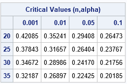
For each sample size, the corresponding row of the table shows the critical values of D for which CDF(D) = 1-α. Of course, a printed table is unnecessary when you have a programmatic way to compute the quantiles.

Summary

Facchinetti (2009) shows how to compute the CDF for the Kolmogorov D distribution for any value of n and D. The Kolmogorov D statistic is often used for goodness-of-fit tests. Facchinetti's method consists of forming and solving a system of linear equations. To make her work available to the SAS statistical programmer, I translated her MATLAB program into a SAS/IML program that computes the CDF of the Kolmogorov D distribution. This article demonstrates how to use the KolmogorovCDF in SAS/IML to compute and visualize the CDF and density of the Kolmogorov D statistic. It also shows how to use the computation in conjunction with a root-finding method to obtain quantiles and exact critical values of the Kolmogorov D distribution.

Blogs