Authors: Ricky Tharrington and Jagruti Kanjia
In this post, you’ll learn how to assess the bias of machine learning models using tools available in SAS Viya 4. As artificial intelligence grows in popularity, the lives of individuals are increasingly impacted by the predictions of machine learning models in ways ranging from ad suggestions on social media to credit application approvals. Regardless of the importance of the scenario, every model application has the potential to affect separate segments of the user population differently. It’s important for data scientists to understand the biases present in their models to take proper mitigating actions if necessary.
A brief introduction to bias
There are many perspectives to take into account when describing bias in data science. Bias can happen during data collection, data processing, sampling, model building, and so on. This post focuses on the bias present in model predictions. This bias can be broken down further into two categories: performance bias and prediction bias.
Performance and prediction bias are both calculated by finding the largest difference in a particular metric between levels of a sensitive variable. The difference is that performance bias is interested in accuracy metrics while prediction bias is concerned with average predictions.
Ideally, a data scientist would like to eliminate all kinds of biases that are important to a particular application. But it should be noted that performance bias and prediction bias are typically opposed to one another in many applications. Mitigating prediction bias often worsens performance bias, and vice versa. When attempting to mitigate bias, it’s up to the data scientist to consult with experts in the relevant field to understand which type of bias is important to mitigate for their problem.
The Titanic data set
This post uses the popular Titanic data set for its examples. These data were chosen due to their familiarity and interpretability. The Titanic data set comprises observations representing passengers aboard the Titanic during its fatal sinking in 1912. The goal of the models in this post is to predict whether a given individual survived the incident.
The Titanic did not have enough lifeboats for everyone on board. Based on the survivors, we know that lifeboat priority was given to women and children first. From the layout of the ship, we know that more expensive cabins were located closer to the lifeboats. These elements together mean that women and high-class individuals survived at a higher rate than men and the lower class. Machine learning models tend to reflect this behavior. In this post, we’ll train some models to predict survival using these data. We will also measure the bias present between the different sexes represented in the data.
Prior to training models on the Titanic data, it’s common to perform some basic feature engineering work. We applied the following SAS DATA step code to the Titanic data to extract information about the passengers’ titles and the deck locations of their cabins.
data titanic; set titanic; /* Title */ Title = scan(Name,2,","); Title = scan(Title,1," "); Title = tranwrd(Title,".",""); /* Deck */ Deck = " "; if Cabin ^= "" then Deck = substr(Cabin,1,1); run; |
Note that we’re not imputing missing values, a common feature of Titanic-based tutorials because we’ll be using a Forest model in SAS Viya. It has excellent support for missing values out-of-the-box.
Bias assessment in Model Studio
Bias assessment in Model Studio in SAS Visual Machine Learning comes in the form of a new section in the Results of a supervised learning model called Fairness and Bias. To view these reports for a particular classification variable, such as Sex, you must select the “Assess this variable for bias” option in the Data tab of a Model Studio project. Once that is done, the Assess for Bias flag for the given variable will indicate the change. This is demonstrated in Figure 1.

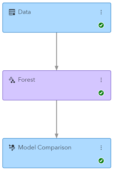
For the purposes of this post, we’ll be creating a pipeline with a single Forest model with all default settings, as demonstrated in Figure 2.
Once the pipeline has been trained, the Bias Assessment report can be viewed by opening a model’s results and selecting “Fairness and Bias." There are a few different plots on this page, but we’ll only be discussing two of them in this post.
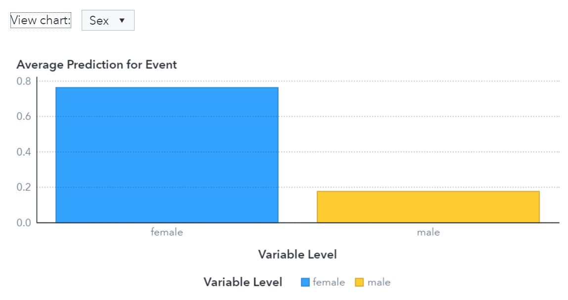
The prediction bias plot for this Forest model, shown in Figure 3, shows the average predicted value for the target event level for this project. In this project, the target event level is “1” indicating whether a passenger survived. The prediction bias plot shows that the average prediction for females is much higher than that of males, meaning that the model predicts a higher survival probability for females than for males. This aligns with our historical understanding of the problem.
The performance bias plot, displayed in Figure 4, shows a few different accuracy metrics for each level of the sensitive variable, Sex. Higher values of True Positive Rate (TPR) and maxKS, and lower values of Multi-Class Log Loss (MCLL) indicate a better fit. All three metrics show that the model’s accuracy is worse for men than for women.

For further information see the Fairness and Bias section of the model results.
These results indicate the model is more accurate for female observations and gives females a higher chance of surviving. Both effects come from the input data, which indicate that women survived the trip aboard the Titanic at a higher rate than men. The Forest model is merely copying this pattern.
Programmatic bias assessment in SAS Viya
Some data scientists prefer training models from SAS Viya’s programmatic interfaces. In this section we’ll repeat the steps from the Model Studio example in Python using the SWAT package.
Forest models are trained by calling the forestTrain action from the decisionTree action set. The following Python snippet trains a Forest model on the Titanic data set like the Model Studio example.
target = "Survived" inputs = ["Pclass","Sex","Embarked","Title", "Deck","Age","SibSp","Parch","Fare"] nominals = ["Survived","Pclass","Sex","Embarked","Title","Deck"] s.decisionTree.forestTrain( table = "TITANIC_TRAIN", target = target, inputs = inputs, nominals = nominal, seed = 12345, maxLevel = 21, nTrees = 1000, encodeName = True, varImp = True, savestate = dict( name = "FOREST_ASTORE", replace = True ) ) |
Once you have a model trained, you can calculate bias statistics by calling the assessBias action from the fairAITools action set. In the Python code below, we calculate bias statistics for the “Sex” variable using our newly trained model.
s.fairAITools.assessBias( table = "TITANIC_TRAIN", modelTable = "FOREST_ASTORE", modelTableType = "ASTORE", predictedVariables = ["P_Survived1","P_Survived0"], response = "Survived", responseLevels = ["1","0"], sensitiveVariable = "Sex" ) |
This is just one possible form of accepted assessBias action syntax. The action can accept scorable models in many different forms including SAS Data Step, DS2, ASTORE, and pre-scored tables. Read more here for examples of calling the assessBias action using a different scoring engine and more details about the results output. Tables 1 and 2 contain a subset of the results from the assessBias action call.
| Sex | MCLL | TPR | PREDICTED_EVENT |
| female | 0.313 | 0.957 | 0.775 |
| male | 0.345 | 0.422 | 0.135 |
Table 1 – Group Metrics for Titanic Forest model
| Metric | Value | Base | Compare |
| Predictive Parity | 0.641 | female | male |
| Equalized Odds | 0.535 | female | male |
Table 2 – Bias Statistics for Titanic Forest model
Table 1 shows a portion of the Group Metrics table output by the assessBias action. Here we can see the values of many different performance metrics for different levels of the sensitive variable, in this case, “Sex”. MCLL and TPR are both better for female observations than for male observations, and the average predicted event value is much higher for females than for males.
Table 2 shows selected rows from the Bias Statistics output table, which gives common names for differences in metrics from Table 1. Predictive Parity measures the difference in the average prediction, and Equalized Odds gives the maximum difference along TPR and FPR (not shown in this example).
These results follow the results from the Model Studio example and are not surprising given our historical understanding of the Titanic.
Bias mitigation through variable omission
Let’s say we’re interested in reducing the model’s bias between men and women. One common practice for achieving reduced bias between groups is to hide that group’s information from the model. One way to attempt to do this is to remove that variable as an input to the model while training. The action in this next Python example eliminates Sex and Title from the input variable lists. Title is omitted because of its strong association with Sex.
s.decisionTree.forestTrain( table = "TITANIC_TRAIN", target = target, inputs = ["Pclass","Embarked","Deck","Age","SibSp","Parch","Fare"], nominals = ["Survived","Pclass","Embarked","Deck"], seed = 12345, maxLevel = 21, nTrees = 1000, encodeName = True, varImp = True, savestate = dict( name = "FOREST_ASTORE", replace = True ) ) |
Here are the same result tables as shown before, but on the new model that did not have access to Sex and Title directly.
| Sex | MCLL | TPR | PREDICTED_EVENT |
| female | 0.522 | 0.695 | 0.514 |
| male | 0.369 | 0.606 | 0.256 |
Table 3 - Group Metrics for Titanic Forest model omitting Sex and Title
| Metric | Value | Base | Compare |
| Predictive Parity | 0.259 | female | male |
| Equalized Odds | 0.090 | female | male |
Table 4 - Bias Statistics for Titanic Forest model omitting Sex and Title
Interestingly, the difference in MCLL between the two groups increased. This seems to be largely caused by a drastic increase in the MCLL for the female group. However, the TPR difference has been reduced significantly, as well as the difference in average predicted event probability.
There are other methods for mitigating bias in machine learning models not covered in this post, such as oversampling or weighting input data based on the sensitive variable. As we know from historical information, Sex was an important factor in determining whether a passenger aboard the Titanic survived. So it follows that accuracy should suffer if the model is not given access to this information. But this demonstrates that it's possible to trade model accuracy for a reduction in bias. This accuracy-bias tradeoff is likely desirable in many situations, especially in high-risk applications.
Conclusion
It’s important to be aware of the different sources of bias in each data science application and the magnitude of their effect on model prediction. In this post, we’ve demonstrated how to assess models built in Model Studio in SAS Visual Machine Learning and directly in the CAS server in SAS Viya. Our hope is that the tools shown in this post will be useful for you when assessing the bias present in your own models.
LEARN MORE | SAS Viya