
The Vehicle Routing Problem (VRP) algorithm aims to find optimal routes for one or multiple vehicles visiting a set of locations and delivering a specific amount of goods demanded by these locations. Problems related to the distribution of goods, normally between warehouses and customers or stores, are generally considered vehicle routing problems.
The VRP was first proposed by Dantzig and Ramser in the paper "The Truck Dispatching Problem," published in 1959 by INFORMS in volume 6 of the Management Science journal. This paper searches for an optimal route for a fleet of gasoline delivery trucks between a bulk terminal and a large number of service stations supplied by the terminal.
The shortest routes between any two locations in the system are given and a demand for one or several products is specified for several stations within the distribution systems. The VRP algorithm aims to find a way to assign stations to trucks in such a manner that the station demands are satisfied while keeping the total mileage covered by the fleet to a minimum.
More complex than the Traveling Salesman Problem
The vehicle routing problem is a generalization of the traveling salesman problem. As with the traveling salesman problem, the solution searches for the shortest route that passes through each location once. A major difference is that there is a demand from each location that needs to be supplied by the vehicle departing from the depot.
The fact that the vehicles have a resource capacity is really what makes VRP so much harder than TSP. Assuming that each pair of locations is joined by a link, the total number of different routes passing through n locations is (n-1)!/2. Even for a small network, or a reduced number of locations to visit, the total number of possible routes can be extremely large.
The example in this case study perfectly describes this scenario. This exercise comprises of only 22 locations (n=22). Assuming that a link exists between any pair of locations set up in this case, the total number of different possible routes is 25,545,471,085,854,720,000. I am not sure if I am even capable of saying this enormous number out loud.
Vehicle routing problems are difficult and computationally expensive to solve. Real-world problems involve various complicating constraints like time windows, time-dependent travel times, multiple depots to originate the supply, multiple vehicles and different capacities for distinct types of vehicles, among others.
Common objective functions for VRP might consist of minimizing the global transportation cost based on the overall distance traveled by the fleet, minimizing the number of vehicles to supply all customers' demands, minimizing the time of the overall travel considering the fleet, the depots, the customers and the loading and unloading times, minimizing penalties for time-windows restrictions in the delivery process or even maximizing a particular objective function like the profit of the overall trips where it is not mandatory to visit all customers.
There are several well-known variants of the VRP that accommodate different combinations of resource contraints, objectives, fleet structure, and routing restrictions. The variant described in this blog is the Capacitated Vehicle Routing Problem (CVRP), where the vehicles have limited capacity to carry the goods to be delivered.
Other variants include:
- The Vehicle Routing Problem with Time Windows (VRPTW) where each location must be served by the vehicles within a particular period of time.
- The Vehicle Routing Problem with Heterogeneous Fleets (HFVRP) where different vehicles have different capacities to carry the goods.
- The Time-Dependent Vehicle Routing Problem (TDVRP) is where customers are assigned to vehicles that are assigned to routes and the total time of the overall routes needs to be minimized.
- The Multi-Depot Vehicle Routing Problem (MDVRP), where there are multiple depots from which vehicles can start and end the routes.
- The Open Vehicle Routing Problem (OVRP), where the vehicles are not required to return to the depot.
- The Vehicle Routing Problem with Pickup and Delivery (VRPPD), where goods need to be moved from some locations (pickup) to other locations (delivery), among others.
Let's optimize delivering beer in Asheville!
The example here is a very simple, although crucial problem that the world depends on... optimizing the beer delivery process! In this demo, we will consider three scenarios: one truck, two trucks and four trucks. For the first two scenarios, consider a medium truck with a capacity for 23 beer kegs. The third scenario considers a bigger truck with a capacity for 30 beer kegs.
There are additional constraints for the scenarios. Each customer location is serviced by only one vehicle. Each customer demand is indivisible. Each vehicle cannot exceed its maximum capacity. Each vehicle starts and ends its route at the depot. There is one single depot to supply goods for all customers. Finally, customer demands, distances among customers, between customers and depot and the delivery costs are all known.
To make this case more realistic and perhaps more enjoyable, let’s consider a real (and awesome) brewery that needs to deliver beer kegs to different bars and restaurants throughout multiple locations. A city that is quite famous for its beer in North Carolina is Asheville. The city is famous for other things, of course. It has a beautiful art scene, gorgeous architecture, a colorful autumn season, the historic Biltmore Estate, the Blue Ridge Parkway, and the River Arts District, among many others.
Asheville also has more breweries per capita than any city in the US, with 28.1 breweries per 100,000 residents. How about that?! I have been to Asheville a couple of times, and this is what amazes me most. My wife loves the autumn greenery and the art scene, my children love the tasty restaurants and I love (as you could probably easily guess) the breweries!
So, I picked real-world places in Asheville, some of which I have been to and some of which I have not (yet). These places are the customers in the case study. For the depot, I picked a brewery that I really like. The problem then has a total of 22 locations, including the depot, plus 21 restaurants and bars. This might seem like a lot, but it definitely is not, especially considering the number of great bars and restaurants in Asheville.
Each customer has its own demand. To start off, let's consider the first scenario involving one single pickup truck with a limited capacity of 23 kegs.
Scenario #1: 1 truck, 23 kegs
The following code creates a list of places with the coordinates and the demand. It also creates the macro variables so we can be more flexible along the way, changing the number of trucks available and the capacity of the trucks.
cas; libname mycas cas sessref=casauto; %let dm = /greenmonthly-export/ssemonthly/homes/Carlos.Pinheiro@sas.com/Asheville; %let depot = 'Zillicoach Beer'; %let trucks = 1; %let capacity = 23; data places; length place $20; infile datalines delimiter=","; input place $ lat long demand; datalines; Zillicoach Beer,35.61727324024679,-82.57620125854477,12 Barleys Taproom, 35.593508941040184,-82.55049904390695,6 Foggy Mountain,35.594499248395294,-82.55286640671683,10 Jack of the Wood,35.5944656344917,-82.55554641291447,4 Asheville Club,35.595301953719876,-82.55427884441883,7 The Bier Graden,35.59616807405638,-82.55487446973056,10 Bold Rock,35.596168519758706,-82.5532906435109,9 Packs Tavern,35.59563366969523,-82.54867278235423,12 Bottle Riot,35.586701815340874,-82.5664137278939,5 Hillman Beer,35.5657625849887,-82.53578181164393,6 Westville Pub,35.5797705582317,-82.59669352112562,8 District 42,35.59575560112859,-82.55142220123702,10 Workshop Lounge,35.59381883030113,-82.54921206099571,4 TreeRock Social,35.57164142260938,-82.54272668032107,6 The Whale,35.57875963366179,-82.58401015401363,2 Avenue M,35.62784935175343,-82.54935140167011,4 Pillar Rooftop,35.59828820775747,-82.5436137644324,3 The Bull and Beggar,35.58724435501913,-82.564799389471,8 Jargon,35.5789624127538,-82.5903739015448,1 The Admiral,35.57900392043434,-82.57730888246586,1 Vivian,35.58378161962331,-82.56201676356083,1 Corner Kitchen,35.56835364052998,-82.53558091251179,1 ; |
Here, we are using an open-source package called Leaflet to show the places and routes on a map. The following code creates an HTML file that can be opened in any browser to invoke Leaflet and show all the places that need to be visited.
filename arq "&dm/places.htm"; data _null_; set places end=eof; file arq; length linha $1024.; k+1; if k=1 then do; put '<!DOCTYPE html>'; put '<html>'; put '<head>'; put '<title>SAS Network Optimization</title>'; put '<meta charset="utf-8" />'; put '<meta name="viewport" content="width=device-width, initial-scale=1.0">'; put '<link rel="stylesheet" href="https://unpkg.com/leaflet@1.7.1/dist/leaflet.css" integrity="sha512-xodZBNTC5n17Xt2atTPuE1HxjVMSvLVW9ocqUKLsCC5CXdbqCmblAshOMAS6/keqq/sMZMZ19scR4PsZChSR7A==" crossorigin=""/>'; put '<script src="https://unpkg.com/leaflet@1.7.1/dist/leaflet.js" integrity="sha512-XQoYMqMTK8LvdxXYG3nZ448hOEQiglfqkJs1NOQV44cWnUrBc8PkAOcXy20w0vlaXaVUearIOBhiXZ5V3ynxwA==" crossorigin=""></script>'; put '<style>body{padding:0;margin:0;}html,body,#mapid{height:100%;width:100%;}</style>'; put '</head>'; put '<body>'; put '<div id="mapid"></div>'; put '<script>'; put 'var mymap=L.map("mapid").setView([35.59560349262985,-82.55167448601539],14);'; put 'L.tileLayer("https://api.mapbox.com/styles/v1/{id}/tiles/{z}/{x}/{y}?access_token=pk.eyJ1IjoibWFwYm94IiwiYSI6ImNpejY4NXVycTA2emYycXBndHRqcmZ3N3gifQ.rJcFIG214AriISLbB6B5aw",{maxZoom:20,id:"mapbox/streets-v11"}).addTo(mymap);'; end; linha='L.marker(['||lat||','||long||']).addTo(mymap).bindTooltip("'||place||'- ('||compress(demand)||')",{permanent:true,opacity:0.75}).openTooltip();'; if place = &depot then do; linha='L.marker(['||lat||','||long||']).addTo(mymap).bindTooltip("'||place||'",{permanent:true,opacity:1}).openTooltip();'; put linha; linha='L.circle(['||lat||','||long||'],{radius:75,color:"'||'blue'||'"}).addTo(mymap).bindTooltip("Trucks='||&trucks||' Capacity='||&capacity||' kegs",{permanent:true,opacity:1}).openTooltip();'; end; put linha; if eof then do; put '</script>'; put '</body>'; put '</html>'; end; run; |
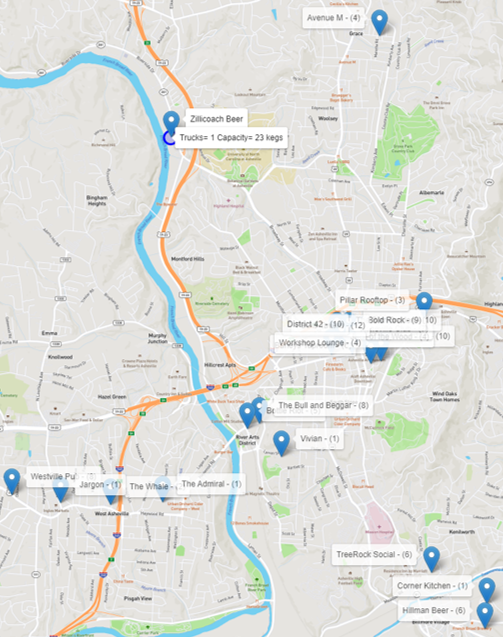
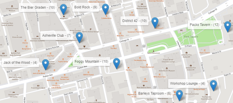
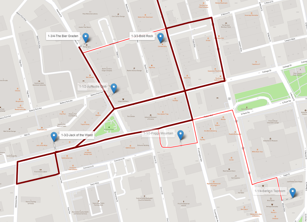
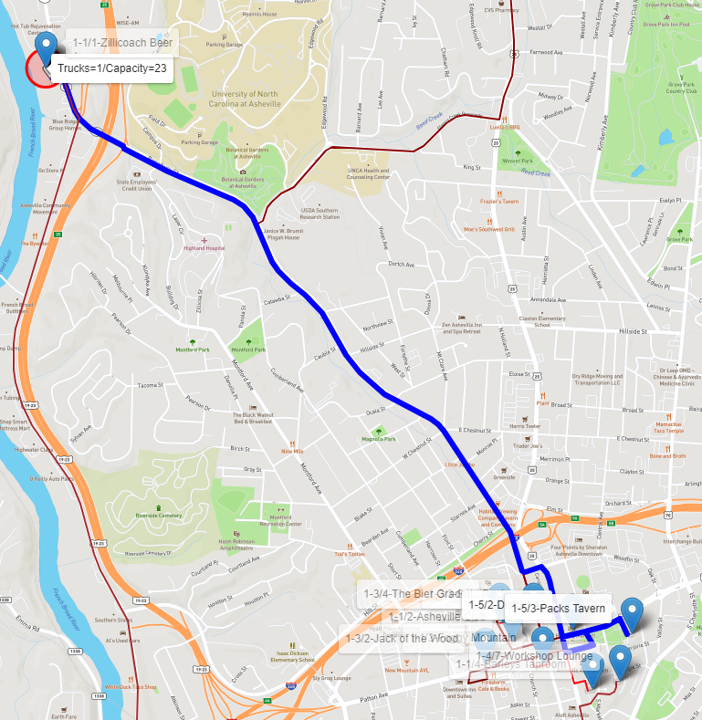
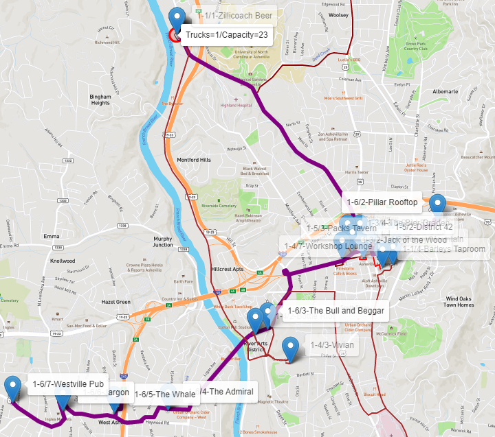
Below is the map with the depot (brewery) and the 21 locations (bars and restaurants) demanding different numbers of beer kegs. Notice the number of beer kegs required by each customer in parentheses. We can see that most of the customers are located downtown.
The next step is to define the possible links between each pair of locations and compute the distances. To simplify the problem, we are calculating the geodetic distance between any possible pair of places; not the existing road distances.
The VRP algorithm will take these geodetic distances into account when searching for optimal routing, trying to minimize the overall distance for the vehicle to travel while delivering the kegs.
The following code shows how to create the links, compute the geodetic distance and create the customer nodes without the depot.
proc sql; create table placeslink as select a.place as org, a.lat as latorg, a.long as longorg, b.place as dst, b.lat as latdst, b.long as longdst from places as a, places as b where a.place<b.place; quit; data mycas.links; set placeslink; distance=geodist(latdst,longdst,latorg,longorg,'M'); output; run; data mycas.nodes; set places(where=(place ne &depot)); run; |
Once the proper input data is set, we can use proc optnetwork to invoke the VRP algorithm. The following code shows how to do this.
proc optnetwork direction = undirected links = mycas.links nodes = mycas.nodes outnodes = mycas.nodesout; linksvar from = org to = dst weight = distance; nodesvar node = place lower = demand vars=(lat long); vrp depot = &depot capacity = &capacity out = mycas.routes; run; |
The following figure shows the result produced by proc optnetwork. It shows the size of the graph, the problem type, and details about the solution.
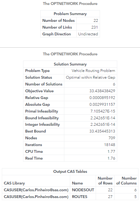
The output table ROUTES presents the multiple trips the vehicle needs to perform in order to properly service all customer demands in terms of beer kegs.
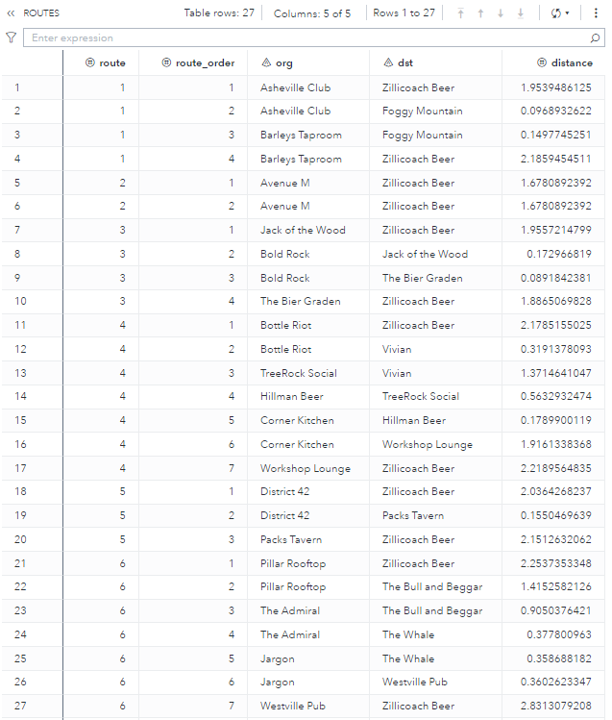
The VRP algorithm searches for an optimal number of trips the vehicle needs to perform and the sequence of places to visit for each trip in order to minimize the overall distance traveled and properly supply all of the customers' demands. A single truck with a capacity of 23 beer kegs will perform 6 trips, eventually going back and forth from the depot to the customers. Depending on the customers' demands and the distances between them, some trips can be really short like route 2 with one single visit to Avenue M, while some trips can be substantially longer like routes 4 and 6 with six customer visits. Click on the map thumbnails below to view them full-sized.
-
- 1. This figure shows the outcomes from the VRP algorithm showing the existing routing plans on a map.
-
- 2. Let’s take a look at the overall routes step by step to better understand what is going on. The first route departs from the brewery and serves 3 restaurants downtown. The truck delivers exactly 23 beer kegs and returns to the brewery to reload more kegs.

-
- 3. The second route in the output table should actually be, at least logistically, the last trip the truck would make, delivering the remaining beer kegs demanded from all the customers. This route has one single customer to visit, supplying only 4 beer kegs.
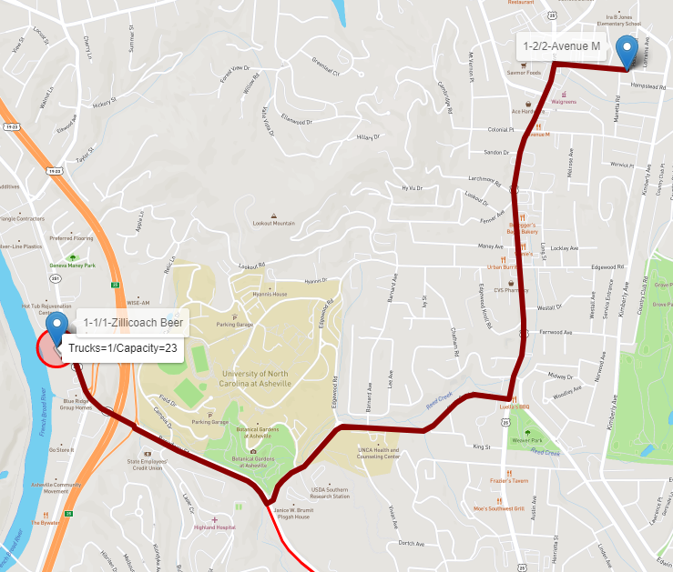
To keep it simple, let’s keep following the order of the routes produced by proc optnetwork. The truck goes from the brewery to Avenue M and delivers, let's say, the last 4 beer kegs to fulfill all the customers' demands.
-
- 4. For the third route, the truck departs from the brewery and serves another 3 customers, delivering exactly 23 beer kegs: 4, 9 and 10, which again, is the maximum capacity of the vehicle.
-
- 5. Notice that the initial route is very similar to the first one, but now the truck is serving three different customers. The following figure shows the delivery process in detail. The thicker dark red line shows the delivery for these new customers.
-
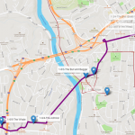
- 6. Once again, the truck returns to the brewery to reload and departs to the fourth route. In the fourth route, the truck serves 6 customers, delivering 23 beer kegs, 5, 1, 6, 6, 1 and 4.
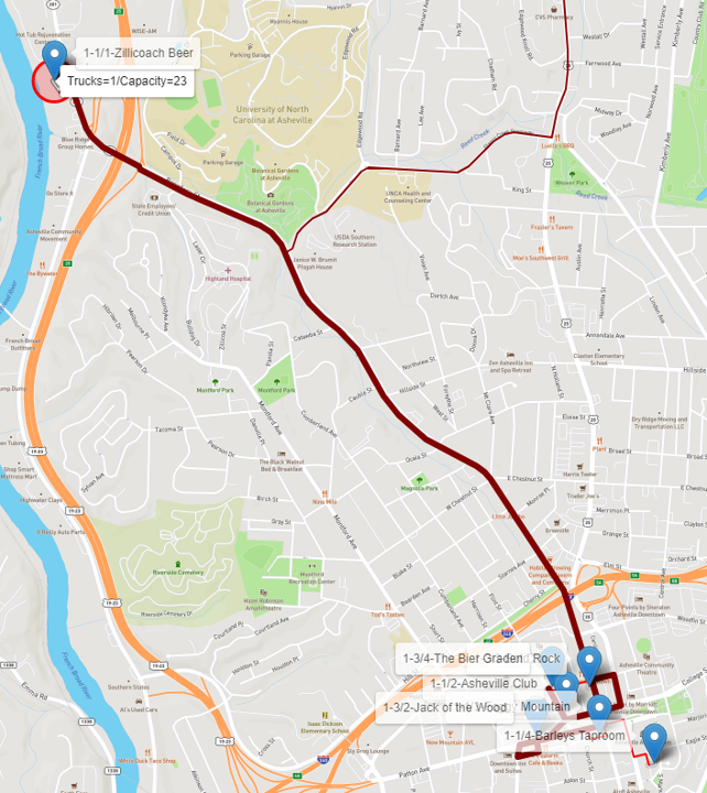
Notice in the following figure that the truck serves customers down south. It stops for 2 customers on the way south, continues on the route serving another 3 customers down there and before returning to the brewery to reload, it stops downtown to serve the last customer with the last 4 beer kegs. The driver must be exhausted! I bet he/she cannot wait to return to the brewery for a cold drink of his/her own. The fifth route is a short one, serving only 2 customers downtown. The truck departs from the brewery; this time not at full capacity because this route supplies only 22 beer kegs: 10 for the first customer and 12 for the second.
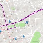
As most of the bars and restaurants are located downtown and the vehicle has limited capacity, the truck needs to make several trips to that region. Notice in the following pictures that all the route lines downtown are differentiated by their color and thickness.
-
- The thicker blue line represents the fifth route serving the customers on this particular trip.
-
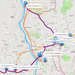
- The last trip serves customers in the western part of the town. However, there is still one customer in downtown to be served. Again, the truck serves 6 customers delivering exactly 23 beer kegs.
-
- Notice that the truck departs from the brewery and goes straight downtown to deliver the first 3 beer kegs to the Pillar Rooftop.

-
- Then, it goes to the western part of downtown to continue delivering the kegs to the other bars and restaurants.
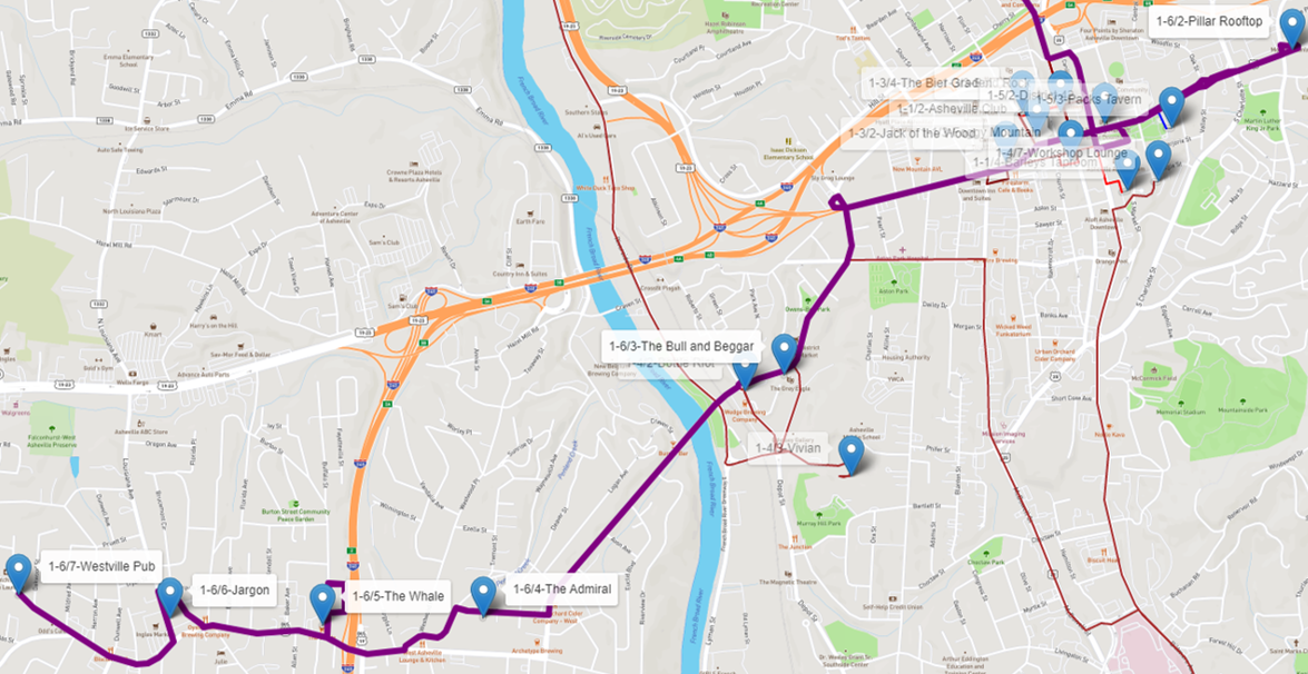
After delivering all the beer kegs and supplying all the customers' demands, the truck completes that route and returns to the brewery.
As we could observe, with only one single vehicle, there are many trips downtown where most customers are located. Eventually, the brewery will realize that they need more trucks or a truck with a bigger capacity to optimize the delivery process. Let’s see how these options work for the brewery.
Scenario #2: 2 trucks, 23 kegs each
For this case study, to simplify the delivery process, we are just splitting the original optimal routes by the number of available vehicles. Few additional steps are added while creating the maps to identify which truck makes a particular set of trips. The following code runs to show multiple trips performed by the available trucks on the map.
proc sql; create table routing as select a.place, a.demand, case when a.route=. then 1 else a.route end as route, a.route_order, b.lat, b.long from mycas.nodesout as a inner join places as b on a.place=b.place order by route, route_order; quit; proc sql noprint; select place, lat, long into :d, :latd, :longd from routing where demand=.; quit; proc sql noprint; select max(route)/&trucks+0.1 into :t from routing; quit; %let trucks = 2; %let capacity = 23; filename arq "&dm/routing.htm"; data _null_; array color{20} $ color1-color20 ('red','blue','darkred','darkblue','black','green','navy','maroon','violet','brown','purple','fuchsia','olive','orange','lime','teal','aqua','gray','silver','white'); length linha $1024.; length linhaR $32767.; ar=route; set routing end=eof; retain linhaR; file arq; k+1; tn=int(route/&t)+1; if k=1 then do; put '<!DOCTYPE html>'; put '<html>'; put '<head>'; put '<title>SAS Network Optimization</title>'; put '<meta charset="utf-8" />'; put '<meta name="viewport" content="width=device-width, initial-scale=1.0">'; put '<link rel="stylesheet" href="https://unpkg.com/leaflet@1.7.1/dist/leaflet.css" integrity="sha512-xodZBNTC5n17Xt2atTPuE1HxjVMSvLVW9ocqUKLsCC5CXdbqCmblAshOMAS6/keqq/sMZMZ19scR4PsZChSR7A==" crossorigin=""/>'; put '<script src="https://unpkg.com/leaflet@1.7.1/dist/leaflet.js" integrity="sha512-XQoYMqMTK8LvdxXYG3nZ448hOEQiglfqkJs1NOQV44cWnUrBc8PkAOcXy20w0vlaXaVUearIOBhiXZ5V3ynxwA==" crossorigin=""></script>'; put '<link rel="stylesheet" href="https://unpkg.com/leaflet-routing-machine@latest/dist/leaflet-routing-machine.css"/>'; put '<script src="https://unpkg.com/leaflet-routing-machine@latest/dist/leaflet-routing-machine.js"></script>'; put '<style>body{padding:0;margin:0;}html,body,#mapid{height:100%;width:100%;}</style>'; put '</head>'; put '<body>'; put '<div id="mapid"</div>'; put '<script>'; put 'var mymap=L.map("mapid").setView([35.59560349262985,-82.55167448601539],12);'; put 'L.tileLayer("https://api.mapbox.com/styles/v1/{id}/tiles/{z}/{x}/{y}?access_token=pk.eyJ1IjoibWFwYm94IiwiYSI6ImNpejY4NXVycTA2emYycXBndHRqcmZ3N3gifQ.rJcFIG214AriISLbB6B5aw",{maxZoom:20,id:"mapbox/streets-v11"}).addTo(mymap);'; linha='L.circle(['||"&latd"||','||"&longd"||'],{radius:80,color:"'||'red'||'"}).addTo(mymap).bindTooltip("Trucks='||"&trucks"||'/Capacity='||"&capacity"||'",{permanent:true,opacity:1}).openTooltip();'; put linha; linhaR='L.Routing.control({waypoints:[L.latLng('||"&latd"||','||"&longd"||')'; end; if route>ar then do; if k > 1 then do; linhaR=catt(linhaR,'],routeWhileDragging:false,showAlternatives:false,reverseWaypoints:false,lineOptions:{styles:[{color:"'||color{route-1}||'",opacity:1,weight:'||10-tn*2||'}]}}).addTo(mymap);'); put linhaR; linhaR='L.Routing.control({waypoints:[L.latLng('||"&latd"||','||"&longd"||'),L.latLng('||lat||','||long||')'; end; end; else linhaR=catt(linhaR,',L.latLng('||lat||','||long||')'); linha='L.marker(['||lat||','||long||']).addTo(mymap).bindTooltip("'||tn||'-'||compress(route)||'/'||compress(route_order)||'-'||place||'",{permanent:true,opacity:0.7}).openTooltip();'; put linha; if eof then do; linhaR=catt(linhaR,'],routeWhileDragging:false,showAlternatives:false,reverseWaypoints:false,lineOptions:{styles:[{color:"'||color{route}||'",opacity:1,weight:'||10-tn*2||'}]}}).addTo(mymap);'); put linhaR; put '</script>'; put '</body>'; put '</html>'; end; run; |
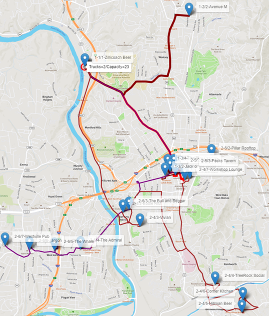
At the top of the map, we can now see the number of trucks (2) and the capacity of the trucks (23) assigned to the depot (brewery). Now, each truck is represented by a different line size. The first routes have thicker lines. The last routes have thinner lines so we can see the different trips performed by the distinct trucks altogether, sometimes overlapping each other.
The first truck runs routes 1, 2 and 3. Route 1 (thicker red) visits 3 customers downtown, identified by the labels 1-1/2-Asheville Club, 1-1/3-Foggy Mountain and 1-1/4-Barleys Taproom. This truck returns to the brewery, reloads and visits route 2 (thicker dark red) for one single customer up north, identified by the label 1-2/2-Avenue M. The truck returns to the depot, reloads and visits 3 other customers on route 3 (maroon), once again downtown, identified by the labels 1-3/2-Jack of the Wood, 1-3-3-Bold Rock and 1-3/4-The Bier Garden. It returns to the depot and stops. In parallel, truck 2 goes southwest on route 4 (brown), visiting 6 customers, labels 2-4/2, 2-4/3, 2-4/4, 2-4/5, 2-4/6 and 2-4/7. It returns to the depot, reloads, and goes through route 5 (violet) to visit 2 customers downtown, identified by the labels 2-5/2 and 2-5/3. It returns to the brewery, reloads and goes through the route 6 (purple) to visit the final 6 customers, 1 to the east, label 2-6/2, 1 to the west, label 2-6/4 and 4 to the far western part of the city, labels 2-6/5, 2-6/5, 2-6/6 and 2-6/7. The trucks return to the brewery and all routes are done in much less time.
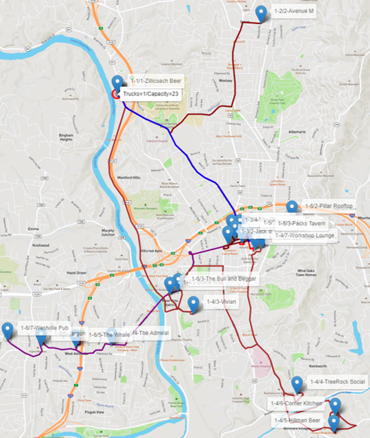
Scenario #3: 4 trucks, 30 kegs each
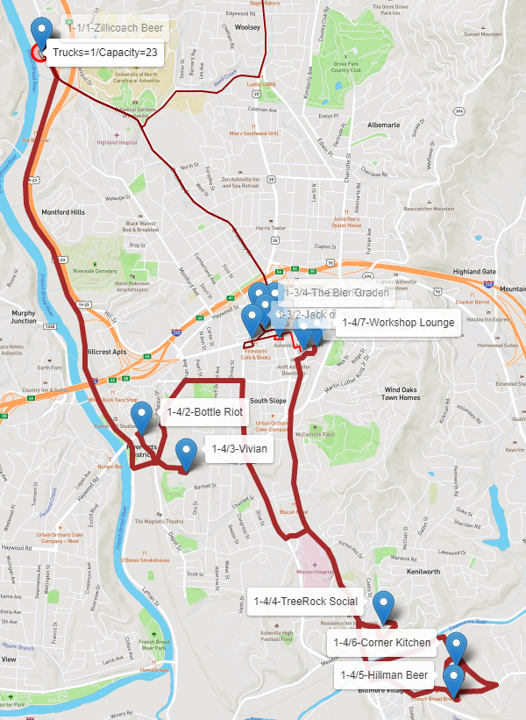
Finally, let’s see what happens when we increase the number of trucks to 4, and the capacity of all trucks to 30 beer kegs. Now, there are only 4 routes and each truck will perform one single trip to visit customers.
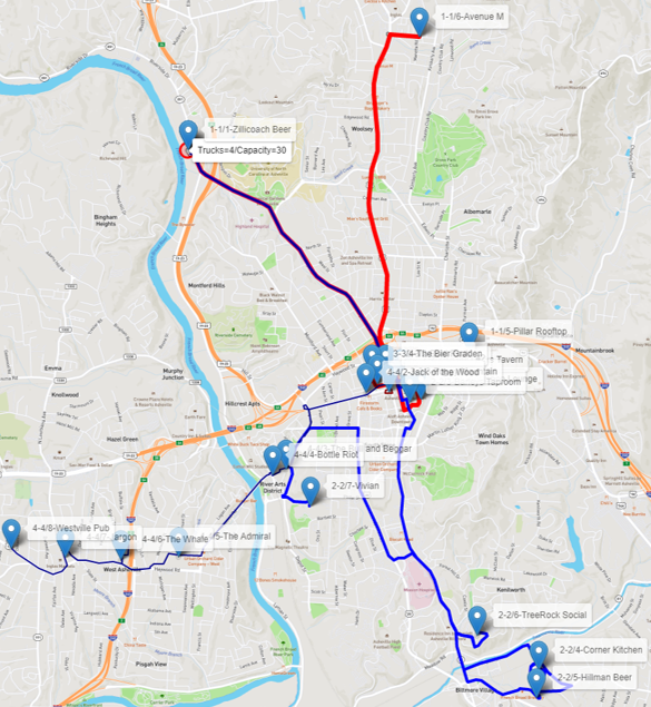
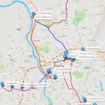
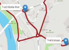
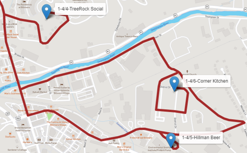
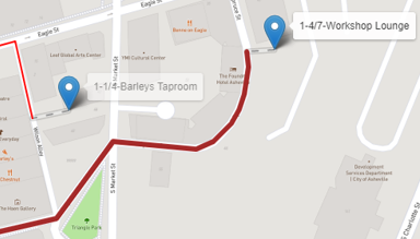
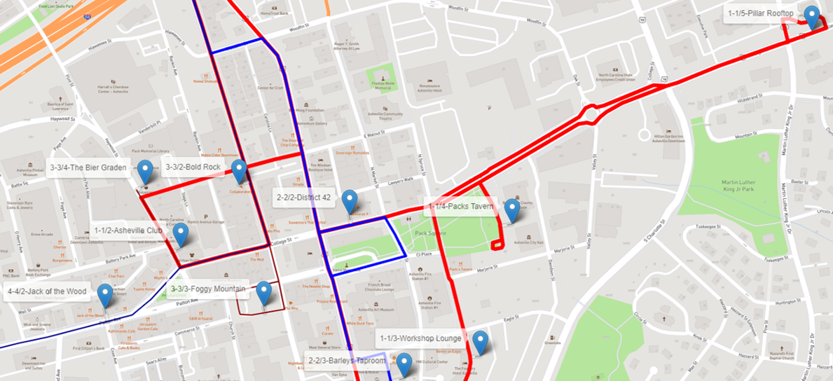
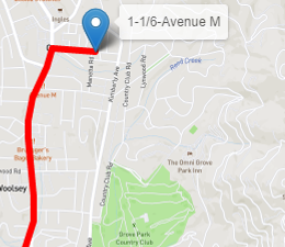
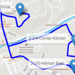
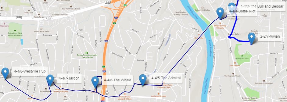
The first truck takes route 1 (red) downtown and to the northern part of the city visiting 5 customers, labeled 1-1/2 to 1-1/6. The second truck takes route 2 (blue) visiting 2 customers downtown, labeled 2-2/2 and 2-2/3, 3 customers in the south, labeled 2-2/4 to 2-2/6 and 1 customer in the west, labeled 2-2/7 before returning to the depot. Truck 3 takes route 3 (dark red) visiting 3 customers downtown, labeled 3-3/2 to 3-3/4. Finally, truck 4 takes route 4 (dark blue) visiting 7 customers in the west and far western part of the city, labeled 4-4/2 to 4-4/8.
-
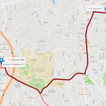
- Downtown is served by trucks 1, 2 and 3.
-
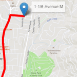
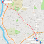
- The north is served by truck 1.
-
- The south is served by truck 2.

-
- The western part of the city is served by truck 4.
Increasing the number of trucks and the capacity of the trucks certainly reduces the time to supply all customers' demands. For example in this particular case study, not considering the time to load and unload the beer kegs and just considering the routing time, the brewery's first scenario with one single truck would take 122 minutes to cover all 6 trips and supply the demands for all 21 customers. In the second scenario with two trucks and the same capacity, the brewery would take 100 minutes to cover all 6 trips, 3 trips for each truck, saving 18% in overall time. Finally, in the last scenario using 4 trucks with slightly more capacity, the brewery would only take 60 minutes to cover all 4 trips, 1 trip for each truck, to serve all 21 customers around the city, saving 51% in overall time.
As you can see, there are plenty of real-world applications (though none as important as beer distribution) for network optimization, particularly around the vehicle routing problem. SAS is continuously improving its network package and adding more and more features. Stay tuned for updates.
Learn more
Thanks for reading. To see more cases in network analysis and network optimization, please check out these links.


2 Comments
From an optimal tour of Brisbane based on a multi-modal transportation system (with a lot of brewery stops) https://blogs.sas.com/content/subconsciousmusings/2021/04/20/brisbane-optimal-tour/ to a vehicle routing problem - a beer distribution example in Asheville... I am seeing two themes here... route optimization and beer!
Another great blog post and analysis Carlos!!!
Thanks Michelle. I guess it is just a coincidence... LOL.